3. Theoretical and mathematical background

3.1. Definitions

3.1.1. Nomenclature

A	=	cross‑sectional area	[m2]
c	=	wave propagation speed	[m/s]
D	=	inner diameter of the pipe	[m]
E	=	Young’s modulus	[N/m2]
e	=	wall thickness	[m]
f	=	friction factor	[‑]
f	=	frequency	[Hz]
g	=	gravitational acceleration	[m/s2]
H	=	Total head	[m]
∆H	=	head loss across the valve	[m]
h	=	elevation of the pipe	[m]
K	=	fluid bulk modulus	[N/m2]
L	=	pipe length, element length	[m]
m	=	mass of the pipe, valve	[kg]
P	=	pressure	[N/m2]
Q	=	discharge	[m3/s]
R	=	inner radius of the pipe	[m]
R	=	hydraulic radius	[m]
s	=	co-ordinate along the pipe	[m]
t	=	time	[s]
uR	=	radial displacement of pipe wall	[m]
V	=	mean fluid velocity	[m/s]
γ	=	elevation angle	[rad]
ν	=	Poisson’s ratio	[‑]
ξ	=	loss coefficient	[‑]
ρ	=	density	[kg/m3]
σ	=	stress	[N/m2]
σφ	=	hoop stress	[N/m2]

3.1.1.1. Superscripts

n

=

time step

3.1.1.2. Subscripts

atm	=	atmosphere
f, F	=	fluid
I	=	place indicator
o, oo	=	steady state
t	=	(pipe), tube
V	=	valve

3.1.2. Bernoulli’s theorem

An important formula to understand the energy terms is Bernoulli’s theorem: it states that the total energy of each particle of a body of fluid is the same provided that no energy enters or leaves the system at a point. The division of this energy between potential, pressure and kinetic energy may vary, but the total remains constant.

Total head = potential head + pressure head + velocity head

In symbols:

\(H=z+\frac{p}{\rho g}+\frac{v^{2}}{2 g}\) (3.1)

In the figure below these terms are explained illustratively (elevation head = potential head) :

Figure 3.1

3.1.3. General definitions

Some definitions are necessary in order to understand the functionality of WANDA. These definitions are used throughout this document and are also important for a proper use of the program.

First we give a summary of general definitions. The general definitions are explained by some examples, which already reveal some of the functionality.

BRANCHED PIPE SYSTEM:

A system consisting of pipes and components connected in an arbitrary way.

HYDRAULIC SYSTEM (H‑system):

The pipe system with respect to the hydraulic components and pipes.

HYDRAULIC MODEL (H‑model):

Mathematical model of an H‑component with respect to its hydraulic features.

HYDRAULIC NODE (H‑node):

Node that connects H‑components via the connect points. The H-node height is the reference level for the pressure in the H-node.

HYDRAULIC COMPONENT (H‑component):

Component defined by its hydraulic properties.

PIPE:

Pipe defined by constant hydraulic properties. The fluid in the pipe is considered as com­pressible. The pipe is in fact a fall type with internal watterhamer nodes.

FALL TYPE:

Type of H‑component, which can be represented by a 2-connect point H‑model. The fluid in the fall type component is considered as incompressible.

SUPPLIER TYPE:

Type of H‑component, which can be represented by a 1‑connect point H‑model. The fluid in the supplier type component is considered as incompressible.

A H-node is represented by one or more connection lines in the diagram. A connection line connects two H-components or a H-component with another connection line.

WATERHAMMER NODE (W‑NODE):

Node in a pipe (not on the extremities). Calculation point of pressure and discharge.

NODAL SET:

Clusters of H-components (fall types and supplier types) at the extremities of the pipes.

WATER LEVEL NODE (S‑NODE):

Even node (0, 2,..) in a free surface pipe in which the water levels are calculated in the staggered grid of the free surface algorithm.

VELOCITY NODE (U‑NODE):

Odd node (1, 3,..) in a free surface pipe in which the fluid velocities are calculated in the staggered grid of the free surface algorithm.

LEVEL, HEIGHT AND OFFSET

In Wanda there are several different inputs used for calculation of elevations. These are:

• Level: This is always relative the reference plane of the case

• Height: This depends upon the component and the manual should be checked to determine relative to which reference the height is taken.

• Offset: This is relative to the h-node elevation unless otherwise specified in the manual.

3.1.4. Examples of systems

In figure 3.2.1 a schematic representation of a pipe system is given. Such a pipe system is often called a ‘branched pipe system’. Several pipes are connected to the same H-node.

Figure 3.2.1: Schematic representation of a pipe system

In figure 3.2.2 a symbolic representa­tion of a simple H‑system is given. The system has four H‑components: two reservoirs, a pump and a check valve, and one pipe. The H-nodes are emphasised by small squares in the figure.

Figure 3.2.2: Schematic representation of a simple pipe system, the H-system

The two reservoirs are supplier types. They are connected to H‑node 1 and to H‑node 4. The pump and checkvalve are fall types. They are located between H‑node 1 and 2, respect­ively H‑node 2 and 3. The difference between supplier and fall types is clear. The supplier types provide the H‑system with fluid. The fall types cause a pressure fall between the H‑nodes.

The pipe has constant hydraulic properties (constant diameter and friction coefficient). There is only one pipe in this system and there are two nodal sets. The first nodal set contains three H‑components. The H‑nodes 1, 2 and 3 all belong to this nodal set. The second nodal set contains only one H‑component and one H‑node.

To be able to perform a transient analysis on the H‑system the pipe must be divided into elements. Suppose we divide the pipe into five elements (figure 3.2.3).

Figure 3.2.3: Schematic representation of the H‑system including the W‑nodes

Then four W‑nodes are introduced. Note that the nodes at the extremities of the pipe are H‑nodes. Once the W‑nodes are defined the H‑system is completely specified.

If the proper data are provided we can perform a transient analysis (steady state and unsteady state).

3.2. Modelling aspects

3.2.1. WANDA Architecture

WANDA is designed such that different domains are covered by one computational core. The architecture is schematically represented in figure 3.3:

• Liquid domain for isothermal fluid flow

• Heat domain for fluid flows with difference in temperature

• Also other domains such as multi-phase flow and mechanics are possible

Figure 3.3: WANDA architecture

Throughout the following chapters the main focus will be on the Liquid-domain, because the other domains in general show much resemblance to Liquid.

3.2.2. Hydraulic components

The symbols in the WANDA diagram are called hydraulic components. The components contain hydraulic models (H-models) which are expressed in mathematical equations. The H‑models define how the variables are related. The number of equations in each H-model depends on the number of connected nodes and the number of core variables in the actual WANDA domain.

For each WANDA domain there is a library of components that can be applied to build the H‑model. Some components in different domains are very similar, such as the pipe or valve in the Liquid or Heat domain. For each domain this manual contains a separate chapter where you can find an extensive physical description of the components.

Each domain contains some components that can be used to define a boundary condition. The component boundh and boundq (Liquid) represent a prescribed head and discharge, whilst the bound pt and bound mt represent a prescribed and temperature-related pressure and mass flow rate (Heat).

3.2.3. Connect point variables

Each Hydraulic component has one or more connect points. For each connect point the main variables (also called the core variables) are calculated. These main variables differs for each domain. Therefore each domain has his own colour of connect point, see the figure below.

Figure 3.4: Similarity between domains

The main variables depends on the actual WANDA domain:

Liquid:

• H (head) [m];

• Q (discharge) [m³/s];

Heat:

• p (pressure) [N/m²];

• M (mass flow) [kg/s];

• T (temperature) [°C];

WANDA uses the main variables to calculate the flow in the pipeline system. Other variables (like for instance fluid velocity or pressure in Liquid models) are derived indirectly from the main variables after the calculation has finished.

The calculations are performed internally in SI-units, but the user can chose the units to use in the Graphical User Interface. WANDA converts the units to SI before calculation and converts it back to the unit system chosen by the user afterwards.

3.2.4. Component phases

Every component can have more than one phase (‘component phase’ or ‘state’). To clarify this concept we take the ideal check valve as an example.

The check valve is a fall type component. It can be in open phase (1st phase) and in closed phase (2nd phase). Both phases are governed by different equations:

phase 1:	check valve is open; Q1 > 0	\(f_{1}: H_{1}=H_{2}\) \(f_{2}: \quad Q_{1}=Q_{2}\)
phase 2:	check valve is closed; H1 < H2	\(f_{1}: \quad Q_{1}=0\) \(f_{2}: \quad Q_{1}=Q_{2}\)

As a result, depending on the component phase, different equations are needed to describe the flow through the check valve. This might seem very trivial, but it is not from the viewpoint of programming, because we do not know a priori when the check valve will close.

The number of phases can be 3, 4 or more depending on the model of the specific component. A pump, for instance, can be in the states: initialisation, running, tripping, starting, turbining etc.

3.2.5. Time dependant actions and control

Some components are active. This means that such components can be activated by the user or by control components. For instance one can close a valve or have a pump trip. One could think that a check valve is also active. This is not true. A check valve closes due to the fluid flow in transient conditions, it cannot be activated by the user in an ‘operative’ sense.

Access to the action tables is only possible in Transient Mode. In an action table the behaviour of that particular component is prescribed in time by the user, e.g. the level in a reservoir, the position of a valve.

With WANDA Control it is possible to simulate operational control loops. As WANDA Control consists of more than 30 logical controllers and numerical functions, there is almost no limitation to the Control circuits in WANDA models.

3.2.6. Calculation types

A distinction can be made between several hydraulic aspects considering time scales. Some component equations have a different form for the steady state and the unsteady state. Therefore, we will distinguish the steady state and the unsteady state.

3.2.6.1. Steady state

Steady state calculations assume that there are no changes in time and all variables are constant. The fluid is considered incompressible. This is the case for instance with computing the appropriate diameter of a pipeline for a given design discharge.

In Engineering Mode WANDA uses only steady state computations.

3.2.6.2. Unsteady state

Unsteady state calculations can be only done in the Transient mode. To start with an unsteady state computation, a correct steady state calculation must be performed thirst.

Figure 3.5: Schematically layout of the WANDA modelling process

Quasi-steady / extended time simulations

Quasi-steady calculations can be considered as a number of independent steady state calculations, which happen to be following each other time. Although the conditions may change with time (e.g. different discharge patterns or valve positions for each time step), each calculation is independent from earlier solutions. For instance engineering tools like Epanet use the quasi-steady approach to determine the water levels and residence time in reservoirs during a certain period of time (day or week).

WANDA uses the quasi-steady approach to calculate the pipe friction at the new time step. WANDA Control uses the quasi-steady approach as it ‘measures’ at the old time step to determine the control-actions at the new time step.

Pressure waves

Due to abrupt changes in the flow conditions (valve closure, filling of pipeline or reservoir) pressure waves develop, which travel through the pipeline (surges). As the fluid and containing pipeline are compressible, the pressure wave needs time to travel from one end of the pipeline to the other end. These pressure waves are very quick phenomena (transients) with wave speeds up to over 1000 m/s.

In Transient mode WANDA calculates the pressure waves in all waterhammer pipes. The fluid in non-waterhammer pipes is considered incompressible, resulting in an infinite wave speed.

Cavitation

Pressure waves and abrupt variations in the pipe profile (e.g. a partially closed valve) can result in substantial changes in pressure. When the fluid pressure drops below the fluid vapour pressure, cavitation can occur. Liquid becomes gas and as gas is more compressible than liquid, the amount of gas in the pipeline changes the flow conditions.

In WANDA the effect of cavitation is included as it recalculates the flow conditions at each time step depending on the pressure and fluid properties.

3.2.7. Solution procedure

The WANDA calculation starts with initialisation and validation of the input. Once the input is validated (e.g. position of check valve is correct), the steady calculation can start (engineering). After the steady calculation has obtained convergence, an unsteady calculation can be performed (transient). All calculations are performed in SI-units. Post processing and conversion to the unit system chosen by the user are part of the Grafical User Interface (GUI) and take place after the calculation of steady (engineering) or the last time step of unsteady (transient). The different steps in the solution procedure of WANDA calculations are schematically depicted in figure 3.6 below.

Figure 3.6: Schematically layout of WANDA Steady and Unsteady solution procedures

In steady state (engineering mode) a start vector is built to start the iteration process. The start vector contains values of the core variables estimated from the input. The friction in all pipes is updated at each iteration.

In unsteady state (transient mode) WANDA uses the solution of the old time step to speed up the calculation process. Dynamic friction and control values are based on the quantities of the core variables at the old time step (quasi-steady).

From a computational point of view the main difference between Engineering and Transient mode is the compressibility of the fluid. As no time-effects are included in Engineering mode, the fluid is considered incompressible and the complete hydraulic set is solved as one big system of equations.

In Transient mode however there is a time-effect due to travel times in the pipes. The non-pipe components (nodal sets) are decoupled, as the wave needs time to travel through the pipe. The decoupled nodal sets are solved as independent systems of equations.

3.2.7.1. Pipe equations

Waterhammer pipes are essential components in wanda. Due to the combined compressibility of the water and containing pipe, there is a delay in exchange of information between the extremities of the pipe. WANDA uses the method of characteristics (see section “Pipes: Method Of Characteristics” on page 159) to calculate the (pressure) waves in the waterhammer pipes. The waterhammer pipes contain internal nodes (W-nodes) where the values of core variables is calculated at each time step.

The total hydraulic set is solved for each time step in the following way. First all waterhammer and free surface pipes are handled such that in every internal node the core variables are computed at t=t+∆t. This results in new values of the core variables at the pipe extremities.

Then all other components are handled as one system of equations. Also ‘rigid column pipes’ are computed here, as the incompressibility causes the information at the extremities to be exchanged instantaneously.

3.2.7.2. System of equations

All equations and variables can be considered together as one system of equations, based on the scheme as build by the modeller. Each component (equation) is therefore related with other components (equations). The model can be represented mathematically by a matrix representing all coefficients of all equations involved. WANDA solves this system of equations for the core variables. This requires the system to have exactly the same number of equations as variables. The components and nodes supply the equations:

• Node equations:

• Mass balance

• Energy balance

• Momentum balance

• Additional (ideal gas law)

• Component equations

• Boundary conditions

• Energy loss

• Wave translation (pipe characteristics)

Since most equations are non-linear (head loss for instance is generally quadratically related to discharge), the equations are linearised in order to solve the system of equations.

3.2.7.3. Number of unknown variables versus number of equations, an example

Suppose we have the following Q-H system:

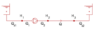
The number of unknown variables is 8: Q_s1, Q₁, Q₂, Q, Q_s2, H₁, H₂, H₃

The number of equations is 8: 2 * 1 boundary condition + 1 * 2 fall eq. + 1 pipe eq. + 3 cont. eq.

The number of unknowns equals the number of equations. Hence, the hydraulic set is completely defined.

3.3. Implementation

Throughout the following the main focus will be on the Liquid-domain, because the other domains in general show much resemblance to Liquid. The core variables are therefore H (head) and Q (discharge).

In steady state the hydraulic set is different in form than in unsteady state. This is caused by the fact that the method of characteristics (MOC) is used to solve the pipe equations, cancelling the direct exchange of information between the extremities of the pipe.

3.3.1. Steady state

3.3.1.1. Supplier type boundary conditions

The basic equation, which governs the steady state of a boundary condition (supplier type) has the general form:

\(f(H, Q)=0\)

(3.2)

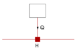
Figure 3.6: Definition of variables for supplier type components,*flow into the system is positive, flow out of the system is negative

H is the head in the node to which the boundary condition is attached. The discharge Q is the discharge that is supplied to the system. The sign convention is: flow into the system is positive, flow out of the system is negative. Most suppliers (air vessel, surge tank) do not supply discharge in steady state. In that case the equation is simply Q = 0. A boundh is a supplier that may supply fluid in steady state as well. The basic equation in steady state is:

H = constant

(3.3)

A supplier type may be non‑linear, but in steady state the basic equation is usually linear.

3.3.1.2. Fall type

The basic equations, which govern the steady state flow through a fall type have the general form (here as an example for a 2-node component):

\(f_{1}\left(H_{1}, \quad H_{2}, \quad Q_{1}, \quad Q_{2}\right)=0\)	(3.4)
\(f_{2}\left(H_{1}, \quad H_{2}, \quad Q_{1}, \quad Q_{2}\right)=0\)	(3.5)

H₁ and H₂ are the pressure heads at the extremities of the 2-node component (see figure 3.7).

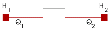
Figure 3.7: Definition of variables for 2-node fall type components

Here we give the valve as an example:

\(f_{1}: H_{1}-H_{2}=c \quad Q_{1}\left|Q_{1}\right|\)	(3.6)
\(f_{2}: Q_{1}=Q_{2}\)

Q₁ is the discharge in the upstream part of the fall type, Q₂ is the discharge in the down­stream part of the fall type. Note that the equations for the valve are non‑linear in Q₁.

Fall type components are usually non-linear. The sign-convention is depending on the symbol representing the component in the WANDA diagram. An arrow, generally from left to right, indicates the positive direction.

3.3.1.3. Pipes: special form of 2-node component

Due to the incompressible behaviour of the fluid in steady state, the discharge is constant along the pipe component. The basic equations, which govern the steady state flow through a pipe are therefore given by the same equations as the other fall-type components. Besides the constant discharge (inflow = outflow) the following equation for the head loss holds:

\(H_{1}-H_{2}-\frac{f L}{D} \frac{Q|Q|}{2 g A_{\mathrm{f}}^{2}}=0\)

(3.7)

The general form of this equation is denoted by:

\(f\left(H_{1}, \quad H_{2}, Q\right)=0\)

(3.8)

Q is the discharge through the pipe. Note that Eq. (3.8) is non‑linear in Q.

H₁ and H₂ are the heads at the H‑nodes of the pipe (see figure 3.8). The Darcy-Weisbach friction factor f in 3.7 above is given by the friction model depending on the flow velocity and properties of the fluid (Newtonian or non-Newtonian), the pipe (diameter, wall roughness). See “Friction models” on page 166 for more information on the friction models in WANDA

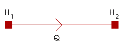
Figure 3.8: Definition of variables for pipes

3.3.1.4. Nodes: Continuity equations

To complete the total hydraulic set, the continuity equations, one for each H‑node, are added. Hence:

\(\sum_{\forall H-n o d e} Q=0\)

(3.9)

It is obvious that these equations are linear. The sign convention is the same as for the boundary conditions. Flow into the H‑node is positive, flow out of the H‑node is negative.

3.3.2. Unsteady state

Boundary conditions are needed to solve the pipe equations using the Method Of Characteristics (MOC). The boundary conditions have to be prescribed at the extremities of each pipe. These boundary conditions are formed by all models in the nodal sets. Therefore, it is necessary to distinguish the equations of the pipes and the so-called nodal set equations.

3.3.2.1. Pipes: Method Of Characteristics

The basic equations, which govern the unsteady state flow through a pipe are usually called the characteristic equations. These equations result from the MOC. A characteristic equation has the general form:

\(C_{H} H+C_{Q} Q=C_{C}\)

(3.10)

and is valid along a characteristic line with either an angle of 1/c_f (C+) or ‑1/c_f (C‑) in the s,t‑plane (c_f is the propagation speed of the pressure waves).

Internal waterhammer nodes

If a pipe is divided into 6 elements, the pipe has 5 W‑nodes. The computational grid of the pipe in the s,t‑ plane is shown in figure 3.9.

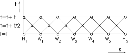
Figure 3.9: Computational grid in transient calculations for a pipe divided into 6 elements. The elements have a constant length ∆s = cf ⋅ ∆t. The characteristic lines cross at nodes denoted with x.

This pipe is described by a total of 12 characteristic equations, one equation for every line. The characteristic lines cross at nodes x. These nodes are neither W‑nodes nor H‑nodes but must be seen as assistance nodes. Suppose that the hydraulic state (H,Q) is known at t=t in every node. First the new H and Q are calculated in the assistance nodes at t=t+(1/2)∆t. Once this is done the new H and Q are calculated in the W‑nodes W₁ ‑ W₅ at t=t+∆t.

As mentioned before, it is not possible to calculate the H and Q at t=t+∆t in H₁ and H₂ by only using the character­istic equations from the specific lines. We also have to know the boundary condi­tions at H₁ and H₂. These boundary conditions are given by the H‑models in the nodal sets. The characteristic equations, which belong to the characteristic lines to the end points of a pipe will be part of the nodal set equations.

The use of assistance nodes is necessary to avoid uncoupled characteristic lines. Such a grid is known as ‘leap frog’. The coefficients for a C⁺ equation are:

CH = 1 CQ = R CC = \(H_{i}^{n}+R Q_{i}^{n}-S Q_{i}^{n}\left|Q_{i}^{n}\right|\)

(3.11)

and for a C^- equation:

CH = 1 CQ = -R CC = \(H_{i+1}^{n}-R Q_{i+1}^{n}+S Q_{i+l}^{n}\left|Q_{i+1}^{n}\right|\)

(3.12)

The upper index denotes time, the lower index denotes place.

3.3.2.2. Other components: Nodal set equations

Every nodal set yields so‑called nodal set equations. The nodal set equations consists of:

1. Equations for the fall type components in the nodal set;

2. Equations for the supplier type components in the nodal set;

3. Continuity equations for every H‑node in the nodal set;

4. Characteristic equations corresponding to the characteristic lines of pipes adjacent to the nodal set.

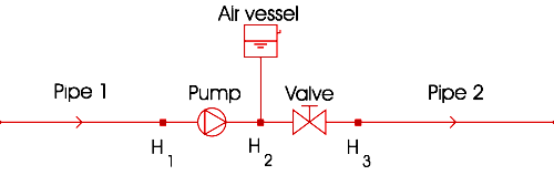
Figure 3.10: An example of a nodal set configuration

In figure 3.10 an example of a nodal set is given. The nodal set consists of two fall types (pump, valve), one supplier (air vessel) and 3 H‑nodes. This nodal set is described by the following equations:

• one characteristic equation for pipe 1

• one characteristic equation for pipe 2

• two equations for the pump

• two equations for the valve

• one equation for the air vessel

• three continuity equations.

Hence the nodal set is governed by 10 equations. Of course the total number of unknown variables is 10 as well:

• discharge of pipe 1

• discharge of pipe 2

• two discharges of the pump

• two discharges of the valve

• one discharge of the airvessel

• three heads at H₁, H₂ and H₃.

As a result the hydraulic behaviour in the nodal set is completely determined. We will discuss now the general forms of all equations except the pipe equations, which we have discussed already.

Fall types

The basic equations, which govern the unsteady state flow through a fall type have the general form (an example for a 2-node component is given):

\(f_{1}\left(H_{1}, \quad H_{2}, Q_{1}, Q_{2}, t\right)=0\)	(3.13)
\(f_{2}\left(H_{1}, H_{2}, Q_{1}, \quad Q_{2}, t\right)=0\)

H₁ and H₂ are the heads at the extremities of the fall type. The discharge Q₁ is defined upstream in the fall type, Q₂ is the discharge downstream in the fall type. The parameter t denotes that other variables in the equation can be a function of time. Here we give an open valve as an example:

\(f_{1}: H_{1}-H_{2}=c(t) \quad Q_{1}\left|Q_{1}\right|\)	(3.14)
\(f_{2}: Q_{1}=Q_{2}\)

The parameter c(t) is a measure of the discharge coefficient of the valve. This coefficient varies in time when the valve is closed or opened. Note that the equations for the valve are non‑linear in Q₁. The fall types are usually non‑linear.

Supplier types

The basic equation, which governs the unsteady state condition of a supplier type has the general form:

\(f(H, Q, t)=0\)

(3.15)

H is the head in the H‑node to which the supplier is attached. Q is the discharge that is supplied to the system. The sign convention is: flow into the system is positive, flow out of the system is negative.

Most suppliers (air vessel, surge tank) supply discharge in unsteady state. A fixed surge tank is governed by the following differential equation:

\(Q=A_{\mathrm{st}} \frac{\mathrm{d} \mathrm{H}}{\mathrm{dt}}\)

(3.16)

in which A_st denotes the area of the surge tank. Such an equation cannot be solved straight­forward, it must be discretised as:

\(Q(t+\Delta t)=A_{\mathrm{st}} \frac{\mathrm{H}(\mathrm{t}+\Delta \mathrm{t})-\mathrm{H}(\mathrm{t})}{\Delta \mathrm{t}}\)

(3.17)

in which ∆t is the time step. This equation is linear in the unknown variables Q and H at t = t+∆t. H at t = t is known. In general a supplier type can be non‑linear as well.

Continuity equations

To complete the nodal point equations the continuity equations must be added for every H‑node in the nodal point. Hence:

(3.3.1)\[\sum{Q}_{\forall H-node} = 0\]

It is obvious that these equations are linear. The sign convention is the same as for the suppliers. Flow into the H‑node is positive, flow out of the H‑node is negative.

3.3.3. Start Vector

3.3.3.1. Steady state

To compute the steady state of the hydraulic set, all equations of the appropriate compo­nent are assembled in one big matrix and one big right hand side vector.

To start the iteration a so‑called start vector must be created by the processor and/or components.

The minimum and maximum number of iterations are defined in the user interface dialogue window “Accuracy window”.

If after the maximum number of iterations the solution has still not been obtained something is badly wrong.

3.3.3.2. Unsteady state

Suppose we have to calculate the first time step. In this case the steady state solution is used as start vector. To solve the next time step we can use the old values of the former time step as start vector. However to speed up the convergence, the procedure after the first time step is slightly different.

In unsteady stat the start vector is filled with new values obtained by extrapolation of the values of the two former time steps, thus for every H‑node in the nodal set:

\(H(t+\Delta t)=\frac{H(t)-H(t-\Delta t)}{\Delta t} \Delta t+H(t) \rightarrow H(t+\Delta t)=2 H(t)-H(t-\Delta t)\)

(3.19)

and for every discharge in the nodal point:

\(Q(t+\Delta t)=\frac{Q(t)-Q(t-\Delta t)}{\Delta t} \Delta t+Q(t) \rightarrow Q(t+\Delta t)=2 Q(t)-Q(t-\Delta t)\)

(3.20)

In this way the start vector for all nodal sets is built.

3.3.4. Linearisation of H-models

During the discussion of the hydraulic set, it appeared that some of the component-models could be non‑linear. A summary of the models with respect to their linear or non‑linear character is given in table 3.3. Again the steady state and unsteady state are distinguished.

Component	Steady state	Unsteady state
Pipe	non-linear	linear
Fall-type	non-linear/linear	non-lin­ear/linear
Supplier-type	non-linear/linear	non-lin­ear/linear

Table 3.3: H‑models classified to linearity

The problem with non‑linear equations is that they cannot be solved by a straightforward algorithm. There are no ‘solvers’ for non‑linear equations. That is why non‑linear equations have to be linearised.

As we can see the component‑model of the pipe in steady state is always non‑linear, whilst in unsteady state the model is always linear. Fall and supplier types can be linear or non‑linear. The linearisation of non‑linear equations is carried out with the Newton‑Raphson method.

3.3.4.1. Linearisation of pipes in steady state

The general form is given by: \(f\left(H_{1}, H_{2}, Q\right)=0\) . Linearisation of this equation results in:

\(f^{i+1}\left(H_{1}, H_{2}, Q\right)=f^{i}\left(H_{1}, H_{2}, Q\right)+\frac{\partial f^{i}}{\partial H_{1}} \Delta H_{1}^{i}+\frac{\partial f^{i}}{\partial H_{2}} \Delta H_{2}^{i}+\frac{\partial f^{i}}{\partial Q} \Delta Q^{i}=0\)

(3.21)

in which:

• \(\Delta H_{1}^{i}=H_{1}^{i+1}-H_{l}^{i}\)

• \(\Delta H_{2}^{i}=H_{2}^{i+1}-H_{2}^{i}\)

• \(\Delta Q^{i}=Q^{i+1}-Q^{i}\)

In this equation i denotes the iteration step. The values subscripted by i are known while the values subscripted by i+1 are to be calculated. Eq. (3.21) can be written in matrix notation in the following way.

Denote:

\(\frac{\partial f^{i}}{\partial H_{1}}=\mathrm{DH}_{1}, \quad \frac{\partial \mathrm{f}^{\mathrm{i}}}{\partial \mathrm{H}_{2}}=\mathrm{DH}_{2}, \quad \frac{\partial \mathrm{f}^{\mathrm{i}}}{\partial \mathrm{Q}}=\mathrm{DQ}\)

(3.22)

Then Eq. (3.21) can be written as:

(3.3.2)\[\begin{split}\left[\begin{array}{lll} \mathrm{DH}_{1} & \mathrm{DH}_{2} & \mathrm{DQ} \end{array}\right]^{\mathrm{i}}\left[\begin{array}{l} \mathrm{H}_{1} \\ \mathrm{H}_{2} \\ \mathrm{Q} \end{array}\right]^{\mathrm{i}+1}=\left[\mathrm{DH}_{1} \mathrm{H}_{1}+\mathrm{DH}_{2} \mathrm{H}_{2}+\mathrm{DQQ}-\mathrm{f}\right]^{\mathrm{i}}\end{split}\]

(3.23)

This equation can be written more conveniently by writing the right hand side as CON:

(3.3.3)\[\begin{split}\left[\begin{array}{lll} D H_{1} & D H_{2} & D Q \end{array}\right]^{i} \left[\begin{array}{ccc} H_{1} \\ H_{2} \\ Q \end{array}\right]^{i+1}=[\mathrm{CON}]^{\mathrm{i}}\end{split}\]

(3.24)

This linear equation is actually to be solved by the computer. Because of the linearisation an iterative procedure is applied. This procedure is called the hydraulic iteration (H‑iteration).

In unsteady state the pipe equations do not have to be linearised. The characteristic equations are already linear. The solution procedure of these equations is completely different from the nodal set equations.

3.3.4.2. Linearisation of fall‑types

The linearisation of the fall‑type equations is the same in steady and unsteady state. The general form is given by:

\(f_{1}\left(H_{1}, \quad H_{2}, Q_{1}, Q_{2}, t\right)=0\)	(3.25)
\(f_{2}\left(H_{1}, H_{2}, Q_{1}, \quad Q_{2}, t\right)=0\)

Linearisation of these equations results in:

(3.3.4)\[\begin{split}\begin{array}{l} f_{1}^{i+1}\left(H_{1}, H_{2}, Q_{1}, Q_{2}, t\right)=f_{1}^{i}\left(H_{1}, H_{2}, Q_{1}, Q_{2}, t\right)+ \\ \frac{\partial f_{1}^{i}}{\partial H_{1}} \Delta H_{l}^{i}+\frac{\partial f_{1}^{i}}{\partial H_{2}} \Delta H_{2}^{i}+\frac{\partial f_{1}^{i}}{\partial Q_{1}} \Delta Q_{1}^{i}+\frac{\partial f_{1}^{i}}{\partial Q_{2}} \Delta Q_{2}^{i}=0 \end{array}\end{split}\]

(3.26)

And

(3.3.5)\[\begin{split}\begin{array}{l} f_{2}^{i+1}\left(H_{1}, H_{2}, Q_{1}, Q_{2}, t\right)=f_{2}^{i}\left(H_{1}, H_{2}, Q_{1}, Q_{2}, t\right)+ \\ \frac{\partial f_{2}^{i}}{\partial H_{1}} \Delta H_{l}^{i}+\frac{\partial f_{2}^{i}}{\partial H_{2}} \Delta H_{2}^{i}+\frac{\partial f_{2}^{i}}{\partial Q_{1}} \Delta Q_{1}^{i}+\frac{\partial f_{2}^{i}}{\partial Q_{2}} \Delta Q_{2}^{i}=0 \end{array}\end{split}\]

(3.27)

Using the same convention for the notation as for the pipe, the linearised equations can be written as:

(3.3.6)\[\begin{split}\left[\begin{array}{cccc} \mathrm{D} 1 \mathrm{H}_{1} & \mathrm{D} 1 \mathrm{H}_{2} & \mathrm{D} 1 \mathrm{Q}_{1} & \mathrm{D} 1 \mathrm{Q}_{2} \\ \mathrm{D} 2 \mathrm{H}_{1} & \mathrm{D} 2 \mathrm{H}_{2} & \mathrm{D} 2 \mathrm{Q}_{1} & \mathrm{D} 2 \mathrm{Q}_{2} \end{array}\right]^{\mathrm{i}}\left[\begin{array}{c} \mathrm{H}_{1} \\ \mathrm{H}_{2} \\ \mathrm{Q}_{1} \\ \mathrm{Q}_{2} \end{array}\right]^{\mathrm{T}+1}=\left[\begin{array}{c} \mathrm{CON}_{1} \\ \mathrm{CON}_{2} \end{array}\right]^{\mathrm{i}}\end{split}\]

(3.28)

in which:

\(\mathrm{D} 1 \mathrm{H}_{1}=\frac{\partial \mathrm{f}_{1}^{1}}{\partial \mathrm{H}_{1}}, \quad \mathrm{D} 1 \mathrm{H}_{2}=\frac{\partial \mathrm{f}_{1}^{\mathrm{i}}}{\partial \mathrm{H}_{2}}, \quad \mathrm{D} 1 \mathrm{Q}_{1}=\frac{\partial \mathrm{f}_{1}^{\mathrm{i}}}{\partial \mathrm{Q}_{1}}, \ldots \text { etc. }\)

and:

\(\mathrm{CON}_{1}=\mathrm{D} 1 \mathrm{H}_{1} \mathrm{H}_{1}^{\mathrm{i}}+\mathrm{D} 1 \mathrm{H}_{2} \mathrm{H}_{2}^{\mathrm{i}}+\mathrm{D} 1 \mathrm{Q}_{1} \mathrm{Q}_{1}^{\mathrm{i}}+\mathrm{D} 1 \mathrm{Q}_{2} \mathrm{Q}_{2}^{\mathrm{i}}-\mathrm{f}_{1}{ }^{\mathrm{i}}\) \(\mathrm{CON}_{2}=\mathrm{D} 2 \mathrm{H}_{1} \mathrm{H}_{1}^{\mathrm{i}}+\mathrm{D} 2 \mathrm{H}_{2} \mathrm{H}_{2}^{\mathrm{i}}+\mathrm{D} 2 \mathrm{Q}_{1} \mathrm{Q}_{1}^{\mathrm{i}}+\mathrm{D} 2 \mathrm{Q}_{2} \mathrm{Q}_{2}^{\mathrm{i}}-\mathrm{f}_{2}{ }^{\mathrm{i}}\)

The linear equation (3.27) is actually to be solved by the computer. Because of the linearisation the equations are part of the hydraulic iteration (H‑iteration).

3.3.4.3. Linearisation of supplier‑types

The linearisation of the supplier‑types is the same in steady and unsteady state. The general form is given by \(f(H, Q, t)=0\) . Linearisation results in:

\(f^{i+1}(H, Q, t)=f^{i}(H, Q, t)+\frac{\partial f^{i}}{\partial H} \Delta H^{i}+\frac{\partial f^{i}}{\partial Q} \Delta Q^{i}=0\)

(3.29)

In matrix notation Eq. (3.29) reads:

(3.3.7)\[\begin{split}\left[\begin{array}{ll} \mathrm{DH} & \mathrm{DQ} \end{array}\right]^{\mathrm{i}}\left[\begin{array}{l} \mathrm{H} \\ \mathrm{Q} \end{array}\right]^{\mathrm{i}+1}=[\mathrm{CON}]^{\mathrm{i}}\end{split}\]

in which:

• \(\mathrm{DH}=\frac{\partial \mathrm{f}^{\mathrm{i}}}{\partial \mathrm{H}}\)

• \(\mathrm{DQ}=\frac{\partial \mathrm{f}^{\mathrm{i}}}{\partial \mathrm{Q}}\)

• \(\mathrm{CON}=\mathrm{DH} \mathrm{H}^{\mathrm{i}}+\mathrm{DQ} \mathrm{Q}^{\mathrm{i}}-\mathrm{f}^{\mathrm{i}}\)

The linear equation (3.29) is actually to be solved by the computer. The equations are updated during the hydraulic iteration (H‑iteration).

3.4. Friction models

Several correlations exist for the modelling of the turbulent wall friction. Each correlation has its own background in a particular field. WANDA 4 supports a wide range of turbulent wall friction correlations for both Newtonian and non-Newtonian fluids. The Newtonian fluid is defined by a constant kinematic viscosity. For laminar wall friction a theoretical wall friction function can be derived: the well-known Poiseulle equation. WANDA supports the following wall friction correlations:

• Theoretical friction according to Darcy-Weisbach

• for Newtonian fluids: Colebrook-White

• for non-Newtonian fluids: Herschel-Bulkley

• Empirical models

• Hazen-Williams

• Chezy-Manning

3.4.1. Theoretical friction models (Darcy-Weisbach)

The steady state pressure drop over a pipe is computed with the Darcy-Weisbach equation and is a function of the pipe dimensions (L and D), velocity U and wall friction f:

\(H_{2}-H_{1}=\frac{f L}{D} \frac{Q|Q|}{2 g A_{f}^{2}}\)

(3.31)

The user has the flexibility to specify a set of local losses (ξ or n*D values) and the number of fittings for each tabulated local loss. These local losses are included in the hydraulic grade line:

\(H_{2}-H_{1}=\left(\frac{f L}{D}+\sum_{i} \xi_{i}\right) \frac{Q|Q|}{2 g A_{f}^{2}}\)	(3.32)
\(H_{2}-H_{1}=\frac{f(L+n D)}{D} \frac{Q|Q|}{2 g A_{f}^{2}}\)	(3.33)

in which:

Q	=	fluid discharge	[m3/s]
Af	=	fluid cross-sectional area	[m2]
D	=	internal diameter of the pipe	[m]
H1	=	upstream head	[m]
H2	=	downstream head	[m]
f	=	Darcy-Weisbach friction factor	[s2/m5]
g	=	gravitational acceleration	[m/s2]
n	=	Equivalent length local loss specification	[-]
ξi	=	Local loss coefficient i	[-]

3.4.1.1. Newtonian fluids: Colebrook-White

The friction Darcy-Weisbach factor f is dependent of the wall roughness k and the Reynolds number Re and is computed with one of the following equations:

\(f=0.64\) for \(0<\mathrm{Re}<100\) ,	(3.34)
\(f=\frac{64}{\operatorname{Re}}\) for \(100<\operatorname{Re}<2000\) ,	(3.35)

and for turbulent flow, when Re > 4000, with the Colebrook-White equation:

\(\frac{1}{\sqrt{f}}=-2 \log \left(\frac{k / D}{3.7}+\frac{2.51}{\operatorname{Re} \sqrt{f}}\right)\)

(3.36)

in which:

\(\operatorname{Re}=\frac{Q D}{v A_{f}}=\frac{Q}{v \pi D}\)

(3.37)

with:

• ν = kinematic viscosity [m²/s]

For 2000 < Re < 4000 f is calculated with a linear interpolation between f calculated with (3.35) for Re=2000 and f calculated with (3.36) and Re=4000.

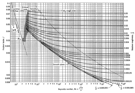
Figure 3.11: Moody-Diagram

Since the Reynolds number is dependent on the fluid discharge, which is to be computed by solving equation (3.33), in which f is present, which in its turn is dependent on the Reynolds number, cyclic dependency occurs. To solve this implicit problem the solution procedure has to be iterative.

The Reynolds numbers of the pipes for which k has been specified (the k-pipes) will initially be computed by substituting the estimated discharges Q (in the start vector) in the Colebrook-White equation (3.36). Subsequently the f‑values of those pipes can be computed by solving equation (3.34), (3.35) or (3.36). Then the steady state computation can be carried out, solving equation (3.33) for all pipes (together with the equations describing the mathematical models of the other H-components and the continuity equations for all H-nodes).

After the computation of the steady state, the Reynolds numbers of all k-pipes are re-computed based on the updated discharges Q and new f-values are computed. The f-values of the pipes for which f has been specified by the user (the f‑pipes) are left unaffected. The steady state computa­tion is then repeated with the current solution vector used as start vector. This procedure is repeated until convergence is obtained.

The f- and k-values of all pipes are output.

3.4.1.2. Wall roughness k-pipes

The k-values are user specified and are generally in the order of 0.1 to 10 mm. They are dependent of material and age of the pipe. A database of k-values belonging to pipe materials may be created.

When the option “Dynamic Friction” is set to “Quasi-steady”, the friction factor f is recalculated for every time step in all calculation points. This calculation is based on the local flow velocity of the previous time step and the input concerning the wall roughness of the pipe. For k-pipes with “Dynamic Friction” set to “none” the f-value and for the other friction models is left unaffected as is the case with f-pipes.

3.4.1.3. Friction factor f-pipes

The friction factor f is user-specified. After finding a converged steady state solution, the k-values of the f-pipes are computed with the following equation:

\(k=3.7 D\left(10\left(-\frac{1}{2 f^{1 / 2}}\right)-\frac{2.51}{N_{\mathrm{R}} \sqrt{\mathrm{f}}}\right)\)

(3.38)

Caution should be taken when using f-pipes, because the f-value depends on the flow and cannot be known beforehand. Other pipe models where f is taken constant during unsteady calculations (k-pipe without dynamic friction and the empirical models) are limited in a similar way. Large values for the wall roughness k are an indication of erroneous application of the friction model. The user is advised to apply another friction model.

3.4.2. Non-Newtonian Fluids

WANDA supports wall friction factors for all homogeneous non-Newtonian fluids with time-independent behaviour. Non-Newtonian fluids are categorized as having time-independent, time-dependent or visco-elastic rheological behaviour. The non-Newtonian fluids with time-independent rheology include:

• dilatant, shear thickening, fluids like sand or a starch suspension,

• pseudoplastic, shear thinning, fluids like polymer solutions, many colloidal suspensions, paper pulp,

• Bingham plastics with a yield stress, like tooth paste or drilling muds and

• Herschel-Bulkley fluid or Generalised Bingham Plastic (GBP), like some mine tailings.

Dilatant, shear thickening	\(\tau_{y x}=K\left(\frac{d u}{d y}\right)^{n} \quad, n>1\)	(3.39)
Pseudoplastic, shear thinning	\(\tau_{y x}=K\left(\frac{d u}{d y}\right)^{n}, n<1\)	(3.40)
Bingham plastic	\(\tau_{y x}=\tau_{y}+K\left(\frac{d u}{d y}\right)\)	(3.41)
Herschel-Bulkley	\(\tau_{y x}=\tau_{y}+K\left(\frac{d u}{d y}\right)^{n}, n>0\)	(3.42)

Equations (39) to (41) show that the Herschel-Bulkley rheological definition generalizes the other non-Newtonian fluids and even Newtonian fluids (n = 1, K = μ, τy = 0). Therefore, the Herschel-Bulkley rheological model is made available in WANDA. The fluid properties that characterise the non-Newtonian fluid (slurry) are specified in the fluid window:

Yield stress, τy

Viscosity coefficient, K

Exponent, n

The following steady state relation for the laminar flow regime can be derived analytically:

\(Q=\frac{\pi D^{3}}{32}\left(\frac{4 n}{3 n+1}\right)\left(\frac{\tau_{w}[1-x]}{K}\right)^{1 / n}\left[1-a \cdot x-b \cdot x^{2}-c \cdot x^{3}\right]\)

(3.43)

where

\(x=\frac{\tau_{y}}{\tau_{w}}=\frac{4 \tau_{y}}{\rho g D \frac{d H}{d x}}\) \(a=\frac{1}{2 n+1}\) \(b=\frac{2 n}{(n+1)(2 n+1)}\) \(c=n \cdot b\)

(3.44)

The laminar friction factor of a Herschel-Bulkley fluid can be derived analytically as well, using the effective viscosity concept:

\(f_{s, l a m}=\frac{64}{\operatorname{Re}_{s}}\) \(\mathrm{Re}_{s}=\frac{v \cdot D}{v_{e q}}\) \(v_{e q}=\frac{g D}{4} \frac{d H}{d x}\left(\frac{4 n}{3 n+1}\right)^{-1}\left(\frac{\tau_{w}[1-x]}{K}\right)^{-1 / n}\left[1-a \cdot x-b \cdot x^{2}-c \cdot x^{3}\right]^{-1}\)

(3.45)

The laminar friction factor does not exceed 6400 for reasons of numerical stability.

If the slurry Reynolds number is greater than 1000, then both the laminar and turbulent friction factor are determined and the maximum of both friction factors is applied. The turbulent wall friction of a Herschel-Bulkley fluid is based on the secant viscosity at the wall and the approach from Wilson and Thomas (1985). Since Wilson and Thomas’ approach is based on a comparison with an equivalent Newtonian fluid, we will use subscripts s for slurry and n for Newtonian properties. The following computations are performed to obtain the turbulent friction factor of non-Newtonian fluids fs,t .

\(\left(\frac{8}{f_{s, t}}\right)^{0.5}=\left(\frac{8}{f_{n, t}}\right)^{0.5}+11.6(\alpha-1)-2.5 \ln \alpha-\Omega\)

(3.46)

Where f_n,t denotes the turbulent friction factor of a Newtonian fluid at the same wall shear stress. Hence the following relation holds between the non-Newtonian and Newtonian friction factors and pipe velocities:

\(\tau_{w, s}=\tau_{w, n} \Leftrightarrow f_{s} \cdot v_{s}^{2}=f_{n} \cdot v_{n}^{2}\)

(3.47)

The two friction factors are computed from the Colebrook-White correlation (see “Theoretical friction models (Darcy-Weisbach)” on page 166) at the wall viscosity μw and Reynolds numbers.

\(\mu_{w}=\frac{\tau_{w, s}}{d v(r) /\left.d r\right|_{w}}=\tau_{w, s}\left(\frac{K}{\tau_{w, s}-\tau_{y}}\right)^{1 / n}\) \(\mathrm{Re}_{s}=\frac{\rho v_{s} D}{\mu_{w}}\) \(\mathrm{Re}_{n}=\frac{\rho v_{n} D}{\mu_{w}}\)

(3.48)

The variable α in equation (46) is the ratio of viscous sublayers of the non-Newtonian and equivalent Newtonian fluid. The variable Ω models the effect of plug flow in the core, due to a non-trivial yield stress τy. Since the shear stress drops linearly towards the pipe centreline for any fluid, the local shear stress always becomes smaller than the yield stress τy (>0) within a certain core region.

(3.4.1)\[\begin{split}\begin{array}{l} \alpha=2 \frac{(1+n \cdot x)}{(1+n)} \\ \Omega=-2.5 \ln (1-x)-2.5 x(1+0.5 x) \end{array}\end{split}\]

(3.49)

Since the variables x, α, Ω, μw are all functions of the wall shear stress τw,s and thus functions of the resulting slurry friction factor, an iterative procedure is required to compute the slurry friction factor. The iterative procedure stops if the relative error in the friction factor has dropped to 1e‑6.

As opposed to Newtonian fluids, there is no transition region between the laminar and turbulent flow regime, because in a non-Newtonian fluid the viscous sublayer is relatively thick at the beginning of the turbulent flow regime (Wilson, Thomas 1985). Therefore, the friction factor at these turbulent flows is relatively small, which explains the absence of the transition region. The applicable friction factor is simply the maximum of the laminar and turbulent friction factor:

\(f_{s}=\max \left\{f_{s, l a m}, f_{s, t}\right\}\)

(3.50)

If the user has specified a non-trivial yield stress τ_y, then a hydraulic gradient may be present in a pipe without any flow. This situation occurs if the following condition is satisfied:

\(\left|\frac{d H}{d x}\right|<\frac{4 \tau_{y}}{\rho g \mathrm{D}}\)

(3.51)

The fluid remains static until the hydraulic gradient exceeds this yield stress criterion.

During a transient event, flow reversal may occur locally in a pipe. The flow reversal may lead to fluid stiffening and activation of the yield stress, if the hydraulic gradient satisfies the yield stress criterion.

3.4.3. Empirical models

The implicit expression of the Darcy-Weisbach friction factor requires an extensive iterative calculation. Therefore empirical expressions such as the Hazen-Williams and Chezy-Manning formulae have become very popular. However the lack of theoretical basis restricts the validity. In WANDA they are included mainly because of their wide application in engineering practice. As the Darcy-Weisbach model is generally considered more accurate and the fast iteration in WANDA cancels its main drawback of implicitness, it is advised to use the Darcy-Weisbach model instead of these empirical models. The Darcy-Weisbach model is valid for all flow regimes and liquids.

The Hazen-Williams formula is the most commonly used headloss formula in the US. It cannot be used for liquids other than water and was originally developed for turbulent flow only.

The Chezy-Manning formula is more commonly used for open channel flow. Each formula uses a different pipe roughness coefficient that must be determined empirically. Table 3.2 lists general ranges of these coefficients for different types of new pipe materials. Be aware that a pipe’s roughness coefficient can change considerably with age.

Material	Hazen-Williams C (unitless)	Manning’s n (unitless)
Cast Iron	130 - 140	0.012 - 0.015
Concrete orConcrete Lined	120 - 140	0.012 - 0.017
Galvanized Iron	120	0.015 - 0.017
Plastic	140 - 150	0.011 - 0.015
Steel	140 - 150	0.015 - 0.017
Vitrified Clay	110	0.013 - 0.015

3.4.3.1. Hazen-Williams

The Hazen-Williams constants are based on “normal” conditions with flow velocities of approximately 1 m/s. This method is only valid for water at ordinary temperatures (4 to 25 °C) and turbulent flow with Reynolds numbers above 10⁵.

3.4.3.2. Chezy-Manning

The Chezy-Manning friction model was mainly derived for uniform steady state flow (open channel flow) and therefore the validity for pipe systems is limited.

\(H_{2}-H_{1}=\frac{4.66 L Q^{2}}{d^{5.33}}\)

(3.52)

3.5. Wave propagation speed

The velocity of the pressure wave in the pipeline depends on the compressibility of the fluid and pipeline itself. The general form of the equation for propagation speed can be written as:

\(c=\sqrt{\frac{1}{\rho\left[\frac{1}{K}+\frac{1}{A} \frac{\partial A}{\partial p}\right]}}\)

(3.53)

In which the bulk modulus of the liquid, K, is related to the density change of the liquid by:

\(K=\frac{\Delta p}{\Delta \rho / \rho}\)

(3.54)

3.5.1. Circular cross-section

For thin-wall pipes of internal diameter D and wall thickness e (i.e. D/e > 10), the propagation speed can be calculated from:

\(c=\sqrt{\frac{1}{\rho\left[\frac{1}{K}+\frac{D}{E e}\right]}}\)

(3.55)

The Young’s Modulus of Elasticity, E, depends on the material of the pipe wall. Here, the expression is given for an idealised case where the restraint factor is taken as unity, assuming the Young’s modulus to be large.

3.5.2. Rectangular cross-section

For non-circular cross sections theoretical wave speeds can be derived from equation 3.57 if an expression can be found for the last term in the denominator. For a rectangular cross-section with width w and height h this term can be written as (ref. E.B. Wylie and V.L. Streeter, Fluid Transients, 1978, McGraw-Hill inc.):

\(\frac{\partial A}{A \partial p}=\frac{w}{e E}+\frac{w^{4} R}{15 e^{3} E h}\)

(3.56)

In (3.55) the first term is the contribution of extension of the pipe wall. The second term is the contribution of the bending of the pipe wall. The ‘rectangular factor’, R, is given by

\(R=\frac{6-5 \alpha}{2}+\frac{1}{2}\left(\frac{h}{w}\right)^{5}\left[6-5 \alpha\left(\frac{w}{h}\right)^{2}\right]\)

(3.57)

with

\(\alpha=\frac{1+(h / w)^{3}}{1+h / w}\)

(3.58)

In practise, however, rectangular pipes may contain fillets (filled corners) to increase the strength and flow properties. In WANDA it is possible to include the effect of these fillets in the wave speed by indicating the size of the fillet (distance to wall). For the bending contribution the width w and height h will be reduced with this fillet-size in the equations above. The fillets are also included in calculation of the velocity via the reduction of the cross-sectional area and wet perimeter. As the fillets will only reduce the flexibility (the fillets themselves are also flexible), the reduction of h and w will not be 100% of the fillet size. Therefore, it is possible to specify the structural contribution of the fillets as a percentage of this h/w reduction. The influence of the fillets on the wave speed can be reduced by lowering the structural contribution.

3.5.3. Reduction of wave speed due to free gas

If there is homogenous distributed free gas in the pipeline, the wave speed is reduced because the bulk modulus is reduced. Equation is then written as:

\(c=\sqrt{\frac{1}{\rho_{m}\left[\frac{1-\alpha}{K}+\frac{\alpha}{p \cdot \gamma}+\frac{1}{A} \frac{\partial A}{\partial p}\right]}}\)

(3.59)

Where α is the volume fraction of gas, γ is the polytropic coefficient of the mixture, and p is the absolute pressure of the gas. ρm is the density of the mixture, which is:

\(\rho_{m}=\alpha \rho_{g}+(1-\alpha) \rho_{l}\)

Where ρl and ρg are the liquid and gas densities, respectively.

Although the effect of the free gas can be significant, the free gas is not taken into account in Wanda. In practice the flow velocity in most systems is not high enough to keep the air evenly distributed. The air bubbles will usually collapse into larger air pockets, which cause different behaviour (multiphase flow).

It should be noted that this only concerns “free” gas in the liquid. Dissolved gas doesn’t influence the wave speed. Due to sudden changes in the pressure, dissolved gas can come out of solution (becomes “free” gas) after a certain incubation period. However, the passage time of the pressure surge is much smaller than the incubation period, which ensures that the pressure surge has passed before the gas can affect the wave speed.

3.5.4. Number of pipe elements

The number of elements in the pipe, n, is calculated by the following equation:

\(n=\frac{L}{c \Delta t}\)

(3.60)

Where L is the length of the pipeline, c is the wave speed and Δt is the time step. If the wave speed is lowered, the number of pipe elements rises.

Entering too low a Young’s modulus can cause the number of pipe elements to exceed the maximum number of pipe elements and Wanda will not allow you to run any computations when this happens. Increasing the time step or the Young’s modulus may remedy this.

3.6. Cavitation

3.6.1. Conceptual Model

The standard water hammer equations are used during the calculation. The absolute pressure P_abs may not drop below the vapour pressure P_v. The vapour pressure is dependent on the fluid and the temperature. However, during a computation it is kept constant.

When cavitation occurs at some point in the pipe, the point becomes a boundary condition for the water hammer equations in the adjacent parts of the pipe. In the spatial distribution of the discharges a discontinuity exists at this boundary. The vapour volume enters in the continuity equation. When this volume again becomes zero, the cavity collapses and the boundary condition vanishes.

3.6.2. Algorithmic Implementation

The water hammer computation is executed in all internal computational points in the pipes (the so-called W-nodes). Sets of two equations in the unknown H_P and Q_P in point P (see figure below). In the equations the H_A, Q_A, H_B and Q_B in points A and B respectively are known. The coefficients R and S are determined by pipe and fluid (liquid) prop­erties.

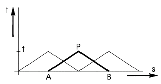
Figure 3.12: Sets of two equations in point P

The equations are:

\(H_{P}-H_{A}+R\left(Q_{P}-Q_{A}\right)+S Q_{A}\left|Q_{A}\right|=0\)	(3.61)
\(H_{P}-H_{B}-R\left(Q_{P}-Q_{B}\right)-S Q_{B}\left|Q_{B}\right|=0\)	(3.62)

with:

\(R=\frac{c_{f}}{g A_{f}} ; S=\frac{\lambda c_{f} \Delta t}{2 g D A_{f}^{2}}\)

(3.63)

and:

\(c_{f}=\frac{1}{\sqrt{\rho_{f}\left(\frac{1}{K}+\frac{D}{E e}\right)}}\)

(3.64)

The following variables are used:

Af	=	fluid cross-sectional area	[m2]
D	=	internal diameter of the pipe	[m]
E	=	Young’s modulus of the pipe	[N/m2]
H	=	head	[m]
K	=	fluid bulk modulus	[N/m2]
Q	=	fluid discharge	[m3/s]
cf	=	water hammer wave speed	[m/s]
e	=	pipe wall thickness	[m]
g	=	gravitational acceleration	[m/s2]
∆t	=	computational time step	[s]
λ	=	Darcy-Weisbach friction factor	[s2/m5]
ρf	=	fluid mass density	[kg/m33]

When at a computational point, H is calculated to be less than H_v, it is simply set equal to H_v. This leads to the following boundary condition:

\(H=H_{\mathrm{v}}\)

(3.65)

where:

\(H_{v}=\frac{P_{v}-P_{a t m}}{\rho_{f} g}+\frac{v^{2}}{2 g}+h\)

(3.66)

is the relative vapour head.

• h = height of computational point relative to the horizontal reference plane

• v = velocity in computational point

• P_atm = atmospheric pressure

Condition (3.63) and the two equations (3.61) and (3.62) now constitute an undetermined system of three equations in the two unknown variables H_P and Q_P. Instead of introducing the void fraction as the third unknown variable, the fluid velocity is assumed to be discon­tinuous at the computational point. The unknown Q_P is replaced by two differing discharges Q₁ and Q₂ up- and down­stream of the “cavitating” computational point. A cavity is now formed, the volume of which is governed by:

\(\frac{\partial V}{\partial t}=Q_{2}-Q_{1}\)

(3.67)

or, when numerically integrated:

\(V(t)=V(t-\Delta t)+\left(\left(Q_{2}(t)-Q_{1}(t)\right) \Delta t\right.\)

(3.68)

The cavity disappears when its volume is calculated to be negative. Then, to satisfy the mass balance, the last positive cavity volume is filled with liquid, according to

\(Q_{1}(t)-Q_{2}(t)=\frac{V(t-\Delta t)}{\Delta t}\)

(3.69)

which is equation (3.68) with V(t) = 0.

In the following figure examples are given for the naming and dependencies of two grid-points: one with cavitation (P) and one without cavitation (Q).

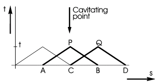
Figure 3.13: Point with (P) and without cavitation (Q).

The system of (uncoupled) equations to be solved in grid-point P is:

\(H_{v}-H_{A}+R\left(Q_{P 1}-Q_{A}\right)+S Q_{A}\left|Q_{A}\right|=0\)	(3.70)
\(H_{v}-H_{B}-R\left(Q_{P 2}-Q_{B}\right)-S Q_{B}\left|Q_{B}\right|=0\)	(3.71)

The system of equations to be solved in grid-point Q is:

\(H_{Q}-H_{C}+R\left(Q_{Q}-Q_{C 2}\right)+S Q_{C 2}\left|Q_{C 2}\right|=0\)	(3.72)
\(H_{Q}-H_{D}-R\left(Q_{Q}-Q_{D}\right)-S Q_{D}\left|Q_{D}\right|=0\)	(3.73)

Characteristic equations in nodal sets

As long as point P in the above example is an (internal) W-node there are no problems. However, when P is at a pipe extremity (end points) it is an H-node. H and Q in these H-nodes are solved in the systems of nodal set equations. After solution of the nodal set equations it may turn out (e.g. in calculation phase 4) that condition (3.65) is not fulfilled. This may be regarded as a change in “procedure phase” of the characteristic equation of the adjacent pipe. The characteristic equation is replaced by: H = H_v thus decoupling the pipe from the nodal set. The Q into that pipe is then separately computed. The cavitation volume V at the H-node must of course being kept track of. The pipe ends are thus regarded as H-procedures with procedure phases “not-cavitating” and “cavitating”.

3.6.3. Software Implementation

The vapour pressure P_v is user specified. The cavitation volume V is component specific output, so it can be selected and plotted. When cavitation occurs within a pipe, the complete vector of cavitation volumes from that pipe is output, so that an animation of the cavitation volumes as function from a route can be pro­duced.

3.7. Pipe models

3.7.1. Pressurised pipe

Compressible fluid: continuity equation is now more complicated for pipes. Fluid in other components is still assumed incompressible as the length scale is much smaller.

Waterhammer pipes are essential components in wanda. Therefore we give a full description of the theory and solution methods.

For the description of an isothermal fluid flow through a pipe two equations are of importance:

• Momentum equation

• Continuity equation.

In water hammer theory both equations are applied on the mean flow. In other words, the flow is considered as one‑dimensional.

Derivation of these one‑dimensional equations can be found in any textbook on transient flow [1, 2, 3].

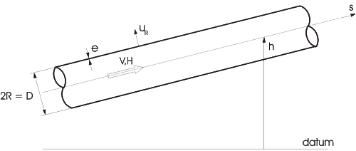
Figure 3.14: Definition of variables

The equations are (see also figure 3.14)

Momentum: \(\frac{\partial V}{\partial t}+g \frac{\partial H}{\partial s}+\frac{f V|V|}{2 D}=0\)	(3.74)
Continuity: \(\frac{\rho_{f} g}{K_{f}} \frac{\partial H}{\partial t}+\frac{\partial V}{\partial s}+\frac{2}{R} \frac{\partial u_{\mathrm{R}}}{\partial \mathrm{t}}=0\)	(3.75)

in which:

V	=	mean velocity	[m/s]
H	=	head	[m]
s	=	axial coordinate (along the pipe)	[m]
g	=	gravitational acceleration	[m/s2]
f	=	friction factor	[‑]
D=2R	=	internal diameter of the pipe	[m]
ρf	=	fluid density	[kg/m3]
Kf	=	fluid bulk modulus	[N/m2]
uR	=	radial displacement of pipe wall	[m]

The head H is defined as:

\(H=\frac{P}{\rho_{f} g}+\frac{v^{2}}{2 g}+h\)

(3.76)

In which P denotes the mean fluid pressure and h the elevation of the centreline of the pipe relative to an arbitrary datum.

Figure 3.15: Hydraulic gradient, pipe elevation, Head and pressure.

Assumptions

• The third term in the momentum equation accounts for the friction between fluid and pipe wall. The friction is modelled the same as if the velocity were steady. This is usually done in transient flow calculations and works out well.

• In the equations (3.74) and (3.75) convective terms like \(V \partial V / \partial s\) are neglected.

  This is allowed only when V is much smaller then the wave speed of the pressure waves. This assumption is known in literature as the acoustic approximation.

• The one‑dimensional description of the fluid flow is only valid for pressure waves with low frequency. One can imagine that if the wavelength of the pressure waves is of the same magnitude as the diameter of the pipe, radial fluid inertia becomes of importance. In transient flow long wavelengths are dominant and a one‑dimensional approach is valid. This assumption is known in literature as the long wavelength approximation [4].

Continuity equation

The continuity equation (3.75) can be transformed in a more convenient form. Therefore we use the stress‑strain relations for the pipe:

\(\frac{u_{\mathrm{R}}}{\mathrm{R}}=\frac{1}{\mathrm{E}}\left(\sigma_{\phi}-v \quad \sigma_{\mathrm{s}}\right)\) \(\frac{\partial u_{s}}{\partial s}=\frac{1}{E}\left(\sigma_{s}-v \sigma_{\phi}\right)\)

(3.77)

or:

\(\sigma_{s}=\frac{E}{1-v^{2}}\left(\frac{\partial u_{s}}{\partial s}+v \frac{u_{\mathrm{R}}}{\mathrm{R}}\right)\) \(\sigma_{\phi}=\frac{E}{1-v^{2}}\left(\frac{u_{\mathrm{R}}}{\mathrm{R}}+v \frac{\partial \mathrm{u}_{\mathrm{s}}}{\partial \mathrm{s}}\right)\)

(3.78)

in which:

E	=	Young’s modulus	[N/m2]
ν	=	Poisson’s ratio	[‑]
σs	=	axial pipe stress	[N/m2]
σφ	=	hoop stress	[N/m2]

By means of the stress‑strain relations the continuity equation can be written as:

\(\frac{\rho_{\mathrm{f}}}{\mathrm{K}_{\mathrm{f}}} \frac{\partial \mathrm{H}}{\partial \mathrm{t}}+\frac{1}{\mathrm{~g}} \frac{\partial \mathrm{V}}{\partial \mathrm{s}}+\frac{2}{\mathrm{gE}} \frac{\partial \sigma_{\phi}}{\partial \mathrm{t}}-\frac{2 v}{\mathrm{gE}} \frac{\partial \sigma_{\mathrm{s}}}{\partial \mathrm{t}}=0\)

(3.79)

This equation can be simplified by applying again the long wavelength approximation.

This approximation states that the radial inertia of the pipe wall can be neglected. If this approximation is applied one can derive an important equation:

\(\sigma_{\phi}=\frac{P R}{e}\)

(3.80)

In fact this equation states that forces in radial direction are always in equilibrium. There are no dynamic effects involved.

Substitution of equation (3.78) in (3.79) yields:

\(\frac{\rho_{\mathrm{f}}}{\mathrm{K}_{\mathrm{f}}} \frac{\partial \mathrm{H}}{\partial \mathrm{t}}+\frac{1}{\mathrm{~g}} \frac{\partial \mathrm{V}}{\partial \mathrm{s}}+\frac{2 \mathrm{R}}{\mathrm{gEe}} \frac{\partial \mathrm{P}}{\partial \mathrm{t}}-\frac{2 v}{\mathrm{gE}} \frac{\partial \sigma_{\mathrm{s}}}{\partial \mathrm{t}}=0\)

(3.81)

The pressure P can be expressed in terms of H by means of equation (3.76):

\(P=\rho_{\mathrm{f}} \mathrm{g}(\mathrm{H}-\mathrm{h})\)

Hence:

\(\frac{\partial P}{\partial t}=\rho_{\mathrm{f}} \mathrm{g}\left(\frac{\partial \mathrm{H}}{\partial \mathrm{t}}-\frac{\partial \mathrm{h}}{\partial \mathrm{t}}\right)\)

In this equation we will neglect the influence of \(\partial h / \partial t\) on \(\partial P / \partial t\) . This can be done if we consider displacements of the pipe small compared to its diameter.

So it appears:

\(\frac{\partial P}{\partial t}=\rho_{f} g \frac{\partial H}{\partial t}\)

(3.82)

Substitution of (3.82) in (3.81) yields the continuity equation:

\(\frac{1}{c_{f}^{2}} \frac{\partial H}{\partial t}+\frac{1}{g} \frac{\partial V}{\partial s}-\frac{2 v}{g E} \frac{\partial \sigma_{s}}{\partial t}=0\)

(3.83)

With:

\(c_{\mathrm{f}}^{2}=\frac{\mathrm{K}_{\mathrm{f}}}{\rho_{\mathrm{f}}}\left(1+\frac{\mathrm{D} \mathrm{K}_{\mathrm{f}}}{\mathrm{E} \mathrm{e}}\right)^{-1}\)

(3.84)

where:

cf	=	Wave propagation speed	[m/s]
Kf	=	Fluid compressibility	[N/m2]
ρf	=	Fluid density	[kg/m3]
D	=	Internal pipe diameter	[m]
E	=	Young’s modulus (pipe elasticity)	[N/m2]
e	=	Pipe wall thickness	[m]

Of course V can be replaced by Q/A_f again to yield the equations in terms of discharge Q and head H. The last term in the continuity equation accounts for the Poisson effect. This term as well as all inertia effects (radial and axial) of the pipe wall is omitted in classical water hammer theory.

Summary

The two basic equations, which describe the compressible flow in a pipe are (in terms of Q and H):

Momentum:

\(\frac{1}{A_{\mathrm{f}}} \frac{\partial \mathrm{Q}}{\partial \mathrm{t}}+\mathrm{g} \frac{\partial \mathrm{H}}{\partial \mathrm{s}}+\frac{\mathrm{f} \mathrm{Q}|\mathrm{Q}|}{2 \mathrm{D} \mathrm{A}_{\mathrm{f}}^{2}}=0\)

Continuity:

\(\frac{1}{c_{\mathrm{f}}^{2}} \frac{\partial \mathrm{H}}{\partial \mathrm{t}}+\frac{1}{\mathrm{~g} \mathrm{~A}_{\mathrm{f}}} \frac{\partial \mathrm{Q}}{\partial \mathrm{s}}=0\)

with:

\(c_{\mathrm{f}}^{2}=\frac{\mathrm{K}_{\mathrm{f}}}{\rho_{\mathrm{f}}}\left(1+\frac{\mathrm{D} \mathrm{K}_{\mathrm{f}}}{\mathrm{E} \mathrm{e}}\right)^{-1}\)

c_f represents the propagation speed of the pressure waves through the pipe, as we will see.

The method of characteristics (MOC)

If we consider H and Q as the dependent variables, the basic equations for the pipe form a set of hyperbolic partial differential equations. This hyperbolic set can be transformed into two sets of ordinary differential equations, which we will denote as C⁺ and C^- equations:

\(\frac{d H}{d t}+\frac{c_{f}}{g A_{f}} \frac{d Q}{d t}+\frac{f c_{f}}{2 g D A_{f}^{2}} Q|Q|=0\) } C+	(3.85)
\(\frac{d s}{d t}=+c_{\mathrm{f}}\)	(3.86)
\(\frac{d H}{d t}-\frac{c_{\mathrm{f}}}{\mathrm{g} \mathrm{A}_{\mathrm{f}}} \frac{\mathrm{d} \mathrm{Q}}{\mathrm{dt}}-\frac{\mathrm{f} \mathrm{c}_{\mathrm{f}}}{2 \mathrm{~g} \mathrm{D} \mathrm{A}_{\mathrm{f}}^{2}} \mathrm{Q}|\mathrm{Q}|=0\) } C+	(3.87)
\(\frac{d s}{d t}=-c_{\mathrm{f}}\)	(3.88)

These equations are usually called the compatibility equations. It must be stated that every solution of this set will be a solution of the original set.

No mathematical approximations have been made.

Finite Difference Equations

To derive the finite difference equations, a “pipe” is divided into equal reaches of ds in length. The time step is chosen equal to \(d t=d s / c_{f}\) .

The equations (3.86) and (3.88) can be represented by straight lines as shown in figure 3.16.

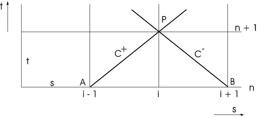
Figure 3.16: The s‑t plane with its characteristic lines C+ and C-

If H and Q are known at point A and B, we can integrate the equations (3.85) and (3.87) along the characteristic lines to point P. After integration the unknowns H and Q in point P can be solved in principle.

Integration yields:

\(\mathrm{C}^{+}: \int_{\mathrm{A}}^{\mathrm{p}} \frac{\mathrm{d} \mathrm{H}}{\mathrm{dt}} \mathrm{dt}+\frac{\mathrm{c}_{\mathrm{f}}}{\mathrm{g} \mathrm{A}_{\mathrm{f}}} \int_{\mathrm{A}}^{\mathrm{p}} \frac{\mathrm{dQ}}{\mathrm{dt}} \mathrm{dt}+\frac{\mathrm{f} \mathrm{c}_{\mathrm{f}}}{2 \mathrm{gD} \mathrm{A}_{\mathrm{f}}^{2}} \int_{\mathrm{A}}^{\mathrm{p}} \mathrm{Q}|\mathrm{Q}| \mathrm{dt}=0\)

(3.89)

\(\mathrm{C}^{-}: \int_{\mathrm{B}}^{\mathrm{P}} \frac{\mathrm{d} \mathrm{H}}{\mathrm{dt}} \mathrm{dt}-\frac{\mathrm{c}_{\mathrm{f}}}{\mathrm{g} \mathrm{A}_{\mathrm{f}}} \int_{\mathrm{B}}^{\mathrm{P}} \frac{\mathrm{d} \mathrm{Q}}{\mathrm{dt}} \mathrm{dt}-\frac{\mathrm{f} \mathrm{c}_{\mathrm{f}}}{2 \mathrm{gD} \mathrm{A}_{\mathrm{f}}^{2}} \int_{\mathrm{B}}^{\mathrm{P}} \mathrm{Q}|\mathrm{Q}| \mathrm{dt}=0\)

(3.90)

The first two terms in the equations can easily be integrated. However, in the last term Q is not known a priori. For this friction term a first order approximation is used.

Integration yields (upper index time, lower index place):

\(\left.H_{i}^{n+1}-H_{i-1}^{n}+R\left(Q_{i}^{n+1}-Q_{i-1}^{n}\right)+S Q_{i-1}^{n}\left|Q_{i-1}^{n}\right|=0\right\} \mathrm{C}^{+}\)	(3.91)
\(\left.H_{i}^{n+1}-H_{i+1}^{n}-R\left(Q_{i}^{n+1}-Q_{i+1}^{n}\right)-S Q_{i+1}^{n}\left|Q_{i+1}^{n}\right|=0\right\} \mathrm{C}^{-}\)	(3.92)

in which:

\(R=\frac{c_{\mathrm{f}}}{\mathrm{g} \mathrm{A}_{\mathrm{f}}} ; \mathrm{S}=\frac{\mathrm{f} \mathrm{c}_{\mathrm{f}} \Delta \mathrm{t}}{2 \mathrm{gD} \mathrm{A}_{\mathrm{f}}^{2}}\)

Then \(H_{i}^{n+1}\) 1 can be expressed in terms of all other variables. Hence:

\(\left.H_{i}^{n+1}=C_{i-1}-R Q_{i}^{n+1} \quad\right\} \mathrm{C}^{+}\)	(3.93)
\(\left.H_{i}^{n+1}=C_{i+1}+R Q_{i}^{n+1} \quad\right\} \mathrm{C}^{-}\)	(3.94)

in which:

\(C_{i-1}=H_{i-1}^{n}+R Q_{i-1}^{n}-S Q_{i-1}^{n}\left|Q_{i-1}^{n}\right|\)	(3.95)
\(C_{i+1}=H_{i+1}^{n}-R Q_{i+1}^{n}+S Q_{i+1}^{n}\left|Q_{i+1}^{n}\right|\)	(3.96)

Ci-1 and Ci+1 both are functions of variables at time tn.

3.7.2. Free surface flow conduit

The free surface conduit is capable of simulating the behaviour of free surface phenomena. The application of this component is useful for simulation of slow filling and draining procedures.

The free surface conduit is capable of handling arbitrary cross sections defined by a table. The cross section table may have a real width (greater than 0) at the top. In this case it is assumed that the cross section is extended with the last entered width.

Waterhammer is not calculated in this component. Consequently the entered time step equals the free surface time step. The grid length of this component is calculated directly from this time step.

\(\Delta x_{F S}=2 \cdot \Delta x=5 \sqrt{g h} \cdot \Delta t_{F S}\)

(3.97)

A free Surface Conduit pipe may be modelled with a closed cross section; a circular cross section for example. This is handled by the free surface algorithm by adding a slot with a width equal to 0.001 times the cross section height and length equal to the grid length. The storage of this slot is used to relate the pressure fluctuation to the flow fluctuation in the completely filled open free surface pipe nodes. Hence the slot storage area of the open free surface pipe is NOT related to the waterhammer wave propagation velocity. Therefore the application of this open free surface pipe in a system with completely filled parts is limited. One should be aware of the way the pressure fluctuations in the completely filled parts are modelled.

The dynamic behaviour of a free surface pipe is described by the continuity and momentum equation.

\(\frac{\partial A(\zeta)}{\partial t}+\frac{\partial}{\partial t}(V A(\zeta))=0\)	(3.98)
\(\frac{\partial}{\partial t}(A V)+\frac{\partial}{\partial x}\left(A V^{2}\right)+g A \frac{\partial H}{\partial x}+g \frac{A V|V|}{C^{2} R}=0\)	(3.99)

in which the Chézy coefficient is related to the pipe friction factor.

\(C=\sqrt{\frac{8 g}{\lambda}}\)

(3.100)

It is assumed that the gas (air) above the free surface in this pipe or channel can enter or leave the pipe freely without causing pressure surges.

The applied numerical algorithm to solve the free surface behaviour, described by equations (3.98) and (3.99), handles all possible free surface flow regimes: sub-critical, super-critical and transitions between both flow types. The numerical algorithm is based on a staggered grid with an upwind computation scheme. The staggered grid has been explicitly imple­mented in WANDA: the algorithm calculates heads in the even S-nodes and velocities in the odd U-nodes. The remaining heads, discharges and other dependent variables are interpolated values. The upwind condition in the numerical scheme guarantees a robust solution, which simulates transitions between sub-critical and super-critical flow regimes.

Slope

The applicability of the continuity and momentum equations for free-surface flow (Saint-Venant equations) is limited to slopes of 1:7 (8 degrees or 14%).

\(\frac{|b(i+1)-b(i)|}{\Delta x_{F S}} \leq 0.14\)

where b(i+1), and b(i) denote the bottom in water level nodes i+1, and i. This criterion is checked in the water level calculation nodes; the boundaries and the even internal calculation nodes are water level nodes.

Slope change

In addition to the maximum slope, the slope change in two consecutive free surface elements is limited. The maximum slope change should be less than 0.14. Formally:

\(\frac{|b(i+1)-2 b(i)+b(i-1)|}{\Delta x_{F S}} \leq 0.14\)

where b(i+1), b(i) resp. b(i-1) denote the bottom in water level nodes i+1, i and i-1. This criterion implies that after an element with maximum slope, the slope in the following element may not be negative. This criterion is checked in the water level calculation nodes.

Element length

The element length of free surface pipes is calculated from the time step. However in Engineering mode the time step is not present. Therefore the user should specify explicitly a maximum element length, which is used in Engineering mode. It is recommended to set this property to 200*D (diameter) or less. In Transient mode the element length is calculated from the time step and it is checked whether the calculated element length is less than the maximum element length. It is recommended to set the maximum element length to 200*D or less, in order to obtain sufficient accuracy.

3.8. Solver Licence

Wanda uses the Lapack numerical library for the matrix solver (http://www.netlib.org/lapack/). The LAPACK library is distributed under the modified BSD license, see the license text below. Note that the modified BSD license text only applies to the LAPACK library, not for the WANDA software.

LAPACK Modified BSD license text:

Copyright (c) 1992-2013 The University of Tennessee and The University of Tennessee Research Foundation. All rights reserved. Copyright (c) 2000-2013 The University of California Berkeley. All rights reserved.

Copyright (c) 2006-2013 The University of Colorado Denver. All rights reserved.

Additional copyrights may follow

Redistribution and use in source and binary forms, with or without modification, are permitted provided that the following conditions are met:

• Redistributions of source code must retain the above copyright notice, this list of conditions and the following disclaimer.

• Redistributions in binary form must reproduce the above copyright notice, this list of conditions and the following disclaimer listed in this license in the documentation and/or other materials provided with the distribution.

• Neither the name of the copyright holders nor the names of its contributors may be used to endorse or promote products derived from this software without specific prior written permission.

The copyright holders provide no reassurances that the source code provided does not infringe any patent, copyright, or any other intellectual property rights of third parties. The copyright holders disclaim any liability to any recipient for claims brought against recipient by any third party for infringement of that parties intellectual property rights.

THIS SOFTWARE IS PROVIDED BY THE COPYRIGHT HOLDERS AND CONTRIBUTORS “AS IS” AND ANY EXPRESS OR IMPLIED WARRANTIES, INCLUDING, BUT NOT LIMITED TO, THE IMPLIED WARRANTIES OF MERCHANTABILITY AND FITNESS FOR A PARTICULAR PURPOSE ARE DISCLAIMED. IN NO EVENT SHALL THE COPYRIGHT OWNER OR CONTRIBUTORS BE LIABLE FOR ANY DIRECT, INDIRECT, INCIDENTAL,

SPECIAL, EXEMPLARY, OR CONSEQUENTIAL DAMAGES (INCLUDING, BUT NOT LIMITED TO, PROCUREMENT OF SUBSTITUTE GOODS OR SERVICES; LOSS OF USE, DATA, OR PROFITS; OR BUSINESS INTERRUPTION) HOWEVER CAUSED AND ON ANY THEORY OF LIABILITY, WHETHER IN CONTRACT, STRICT LIABILITY, OR TORT (INCLUDING NEGLIGENCE OR OTHERWISE) ARISING IN ANY WAY OUT OF THE USE OF THIS SOFTWARE, EVEN IF ADVISED OF THE POSSIBILITY OF SUCH DAMAGE.

3.9. References

1. Wilson, K.C., Thomas, A.D., 1985, A new analysis of the turbulent flow of non-Newtonian fluids, Can. J. Chem. Eng., vol. 63 (pp. 539 – 546).

2. Streeter, V.L., Wylie, E.B., 1978: Fluid Transients. McGraw‑Hill, New York.

3. Fox, J.A., 1977: Hydraulic Analysis of Unsteady Flow in Pipe Networks. MacMillan Press Ltd., London.

4. Chaudhry, M.H., Yevjevich, V., 1981: Closed‑Conduit Flow. Water Resources Publications.

5. Lin, T.C., Morgan, G.W., 1956: Wave propagation through fluid contained in a cylindrical elastic shell. Journal of the Acoustic Society of America, Vol. 28, no. 6, pp. 1165‑1176.

6. Stelling, G.S., Numerical methods for flooding of dry land, Journal of ASCE Hydraulics engineering, 1998

7. Ven Te Chow, Ph.D., 1973: Open Channel Hydraulics. McGrow-hill book Company, New York. ISBN 0-07-085906-X

8. 13. Hnif Chaudhry, Open-Channel Flow, 1993, Prentice Hall, Inc. ISBN 0-13-637141-8

9. http://www.netlib.org/lapack/