2. User Interface
2.1. Overview of WANDA 4 features
2.1.1. MSOffice look and feel
Multiple documents support.
Full drag and drop support.
Full clipboard support.
MS office like tool bars.
MS office like menus.
2.1.2. Diagrams
Wanda 4 uses iGrafx FlowCharter 2017 as diagram engine.
Full drag and drop support.
Copy and move objects and their data between one or multiple documents.
Clipboard support to Word/Excel.
Export a diagram to HTML.
Export a diagram to AutoCAD.
Export a diagram to Visio.
Enhance a diagram with your own text and drawings.
Multiple layer support (you can hide and protect layers easily).
Use your own pictures/maps as background (bmp, gif, autocad, coreldraw, wmf).
Different line styles / weights / colours supported.
Zoom support.
Quick zoom to selection.
Auto fit your printed diagram to m-by-n pages.
Direct feedback to the user. The diagram is real-time validated.
Components with empty/incorrect properties can be easily selected. The diagram window scrolls automatically to the invalid component if the component is out of side.
Vector based and object based schematisation.
Components including connection lines are automatically rotated when you add them in vector based mode.
Hydraulic nodes are automatically recognised. Multiple lines that are connected to each other are recognised as one single calculation node.
Custom-made shape libraries. Deltares can design shape libraries with customer specific components. You can use different shape libraries simultaneously.
Protect your diagrams and properties by a password.
Optionally visible grid.
Optionally snap objects automatically to grid.
2.1.3. Routes in diagram
You can quickly select a route/path through your diagram by selecting the first and last component in the route.
You can quickly ‘align to line’/’rotate’/’reverse a route’.
Selections that contain an unambiguous sequence of pipes are automatically recognised as route.
Selections and routes can be stored using a keyword.
You can see simultaneously an unlimited number of (moving) chart series of different routes.
You can see the overall extremes and total length of a route.
You can build routes with different pipe orientations (results are automatically ‘flipped’)
2.1.4. Automatic name generation
Components and connections are automatically named.
If you assign a name that already exists or if you copy an existing component a new unique name based on the existing name is assigned to the new component. If the name ends with a number, this number is increased, otherwise a character is added to the name.
You can rename a selection of components / connections with a single mouse click.
2.1.5. Property text boxes
View properties (input and output) of hydraulic components directly in text boxes in the diagram.
You can visualise output directly in the diagram for the active time step (see How to use the Time Navigator).
You can visualise output extremes directly in the diagram.
You can specify the properties that you want to see in the diagram.
You can easily move property text boxes in the diagram.
Property text boxes are always attached to a component or connection. Text boxes are automatically moved/deleted/copied when the component or connections moved/deleted/copied.
Property text boxes are placed in a separate layer. This layer can be made hidden. When this text layer is active you can easily move and change the font attributes of those property text boxes.
Property text boxes are also visible when you print the diagram.
The properties ‘Comment’, ‘Model name’ and ‘Reference ID’ (for pipes only) have been included to support a traceable modelling in accordance with ISO 9001.
2.1.6. Property list windows
The main property window displays the properties of all components and connections in diagram selection.
You don’t have to open a separate dialog every time you want to inspect/edit an object. The main property window is instantly adjusted when the diagram selection changes.
You can simply select one or more objects and view/edit this objects at once.
You can open an unlimited number of extra property windows that show a single object.
Input and output together in one list.
You can choose to see the output for the active time step (see How to use the Time Navigator) or to see the extremes in the simulated time period.
Drag and drop support between two property lists.
Easily select properties in the same way you select files in a file manager/explorer. A property that you edit is automatically selected.
Quick synchronisation of selected properties between objects.
Easily compare properties (and tables) from two or more hydraulic components (different values are highlighted in red).
Direct access to all tables from the property list of a hydraulic component with one mouse click.
Write the selected properties to a template file.
Easily change properties by loading a template file (or dropping a template file in the property list window). The loaded properties are automatically selected/highlighted. If you have loaded the wrong template file you can simply press the undo button.
Easily connect you own programs/databases to the property list by using the clipboard or template files.
Opening a time or location chart of one property by pressing the chart button of a property.
Add a property to a chart by dragging a chart button to any chart you like.
Enter values with other units than the active unit group.
View the property value in every available unit for the property dimension at once.
Optionally hide the input or output data.
Overall view of all the selected components. In this view you see the (extreme) values of all the properties available in the selected components.
Change the component type without losing the property values and tables.
Rollback/Undo support.
User name property. The name of the user that made a change to a component is added to the user name property of the changed component.
Modified property. This property shows the last date/time the selected component was changed.
2.1.7. Table editor
The table data can be visualised in a chart next to the table. This chart is automatically updated while you are typing.
Easy adding or removing (multiple) rows.
Clipboard support within one table editor.
Clipboard support between two table editors.
Clipboard support between one table editor and Excel/Word.
Simple numerical operations (+, -, x, /) to a range of table values.
Auto fill missing values by linear interpolation.
Print management.
2.1.8. Spreadsheet
Spreadsheet can be used to edit or view properties of several components simultaneously.
Create a spreadsheet of the diagram selection and selected properties in the property window by one single mouse click.
Unlimited number of different spreadsheets from one or more documents.
Components are sorted by type and name.
Column width is automatically adjusted to fit all values.
You can transpose the spreadsheet. This way you can display components side by side as well as above each other.
You can display extreme values instead of the values of the active time step (see How to use the Time Navigator).
When you print a spreadsheet you can automatically fit to m-by-n pages (portrait and landscape).
Print headers and footers are automatically updated.
You can copy a selection to Excel using the clipboard.
Navigation coupling between spreadsheet and diagram.
2.1.9. Calculations
Fast calculations.
Change something and see the impact of that change in all open windows.
Stop and resume transient calculations.
You can stop a transient calculation before the simulation has ended. When the calculation is stopped you can see the results so far. You can change action tables to interact with the results before you continue the calculation.
Background calculations. While a calculation is in progress you can inspect the running document or continue with another document.
You can calculate multiple documents sequentially (like printer jobs).
Create child cases from parent case
Repeat calculations with varying some input parameters as defined in a simple parameter script; specified output summarised in compact table
You can disuse components temporarily instead of deleting them from the diagram. It is possible to hide parts of the diagram for the calculation kernel. Disused components are greyed out in the diagram. You need one look to see the differences between variants, if you disuse components instead of deleting them.
2.1.10. Chart engine
Drop multiple series (from different documents) into the chart.
Moving location series supported (picture for active time step, see How to use the Time Navigator).
Frozen location series supported. Frozen series show one fixed time step.
Chart time cursor. A vertical blue line gives the active time step in time charts (see How to use the Time Navigator).
View as many charts simultaneously as you want
All open charts support moving series and are automatically updated when input or output is changed.
Create your own custom dedicated chart templates.
Export the chart data to a spreadsheet using the clipboard.
Export the chart to a WMF/JPG/BMP/GIF picture.
Paste the chart in Word using the clipboard.
Series are automatically removed when the (belonging) hydraulic component is deleted or the document is closed.
The chart is automatically closed when it is empty.
Zoom and scroll supported by mouse.
Chart headers and chart footers are automatically updated.
2.1.12. Unit groups
Quickly switch between different unit groups.
All property lists, tables, tabular views and charts are immediately adjusted to the active unit group.
User customised unit group.
2.1.13. Selection builder
Quickly (de)select components/connections by a property, value and operator (<, <=, =, <>, >=, >, like).
Existing keywords, component types, model names and user names are listed by a drop down list.
Add/Remove keywords to/from a selection.
Smart zoom/scroll. If not every selected object is visible the view extend is adjusted to see every selected object.
2.1.14. ‘On demand’ data loading / Smart saving
Quick access to output data of existing documents.
Complicated documents with large output data (100Mb) are loaded within seconds.
Changes are only saved at the moment you save explicitly. If your computer goes down your last saved documents are unchanged/undamaged.
Only changes are saved. This makes it possible to save slightly changed large documents within a second.
2.1.15. Instant window/view refresh
Every (implicit) change is directly reflected in all open views (diagrams, property lists, tables, tabular views and charts).
Any recalculation is directly reflected in all open views. You do not have to reselect your output after recalculation.
2.2. Getting Started
2.2.1. Hydraulic analysis - Functional steps
Examining a hydraulic study of a pipeline system depends on the objectives of the study. A typical sequence is shown in the diagram beneath.
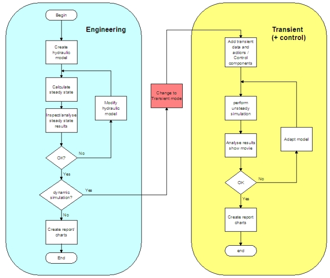
In Engineering mode only so-called steady state calculations can be performed. You have no access to the unsteady state simulation to carry out dynamic phenomena. Only input parameters necessary for the steady state (resistance) calculations must be entered. Changing to Transient mode (menu bar: model/change mode & options) all additional data for the unsteady state becomes accessible.
Opening a new document; it always start in Engineering mode
2.2.1.1. Create the hydraulic model
The first step is to create the schematic diagram of the pipe system and enter component specific hydraulic input data such as geometry, size and other characteristics. This is called “the hydraulic model”. It must be completed successfully before the user may proceed with the actual computation of steady and transient flow.
The most essential function of this part is the conception of the hydraulic model and input of the component specific hydraulic data.
The hydraulic model is in fact a schematic drawing of the actual pipe system, using lines and easy-to-read symbols that represent different elements in the system. It defines all the components in the pipe system with respect to their class and the way they are connected. The conception of the model is realised in the diagram user interface and is fully mouse-operated. WANDA has been designed in such a way that a model can be created with minimum efforts.
The numerical hydraulic data specific to each component are entered via the property windows.
2.2.1.2. Calculate steady state
WANDA computes the steady state. The results are used as the initial conditions for the computation of the unsteady state. steady has no dialogue with the user.
2.2.1.3. Specify hydraulic actions
(Applicable to WANDA Transient only; change to Transient mode using menu model/ mode & options)
In WANDA one can specify the total simulation time and hydraulic actions. Hydraulic actions, such as manipulation of a valve, pump trip or prescribed changes in pressure head or delivery rates, cause hydraulic transients.
Actions are specified in the property window of the particular H-component.
2.2.1.4. Calculate transient
(Applicable to WANDA Transient only; change to Transient mode using menu model/ mode & options)
WANDA also computes the transient flow. This is a separate task. If you unhide this task form the taskbar, the progress in computation including logging messages can be monitored. The estimated time for the simulation is displayed in the header (caption) of the diagram window. The user can interrupt the computation at any time. An interrupted computation can be resumed later on using the same simulation.
During the unsteady calculation the “real time” results can be followed. The user opens the selected graphic windows before starting a calculation. The graphics in these windows are regularly refreshed during the calculation (refresh time is set in model/time window). Looking to the progressing results, you can interrupt the simulation when you find them unsatisfactory. For example, when you evaluate a control system the behaviour of the control can be followed during the simulation. This way it is possible to reduce the simulation time.
Editing data after a calculation all old results remain visible, however coloured differently, and with a strike-through value.
2.2.1.5. Get results
WANDA has powerful utilities to show results. Selected data can be printed in standard report format. Location and/or time series can be put into charts and the dynamic flow process can be visualised using an internal movie feature. The data report and the charts can be displayed on screen, saved on disk or directly sent to the printer.
Printed data report
Printed data are useful for inspection of numerical values of calculated variables. The input and output report are adequately organised in a spreadsheet view, such that it can be included in any formal documentation of a waterhammer simulation.
Charts
These are useful for examining how the pressure or discharges vary as a function of time or along the pipes. Pressure waves travelling along the pipe system are easily recognised from a graph. Selection of the variable and settings of the chart are menu operated and require minimum effort.
The movie feature
The movie is used to visualise the dynamic behaviour of pressures and discharges along selected routes in the pipe system (see Time Navigator).
When the steady and transient state computations are completed, the user might sometimes not be interested in the absolute numbers of calculated variables. He may first want to get some insight into the physical flow process. Animated view of the flow variables using the movie feature will prove to be quite helpful for that purpose. Furthermore the extreme values are displayed in the movie chart. The movie can be recorded and save as AVI-file.
2.2.2. WANDA 4 - User Interface
In this section we will briefly explain how to use together the Component Gallery, the Property Window and the Diagram, in the construction of a hydraulic model.
See also:
Manual/Help iGrafx FlowCharter 2017
2.2.2.1. Introduction
When you start the application you see a screen that can be divided in three major parts.
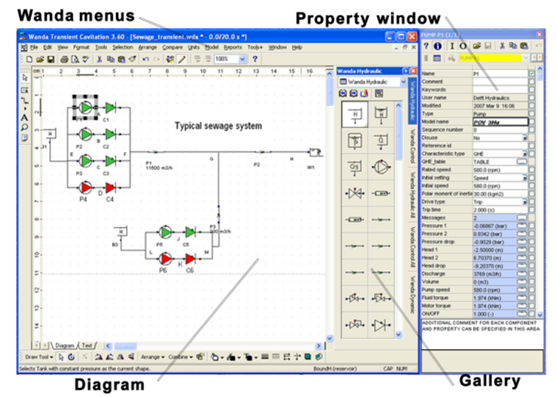
The Diagram in your first session will be empty of course.
The Diagram is the area where you will actually build the hydraulic model that you wish to calculate (see Building the diagram). You will build this model adding components from the Shape Library / Gallery.
The menu bar contains:
iGrafx Flowcharter menus (file/edit/view/insert/format/tools/arrange/window) and
WANDA menus (Selection/Compare/Units/Model/Report/Help).
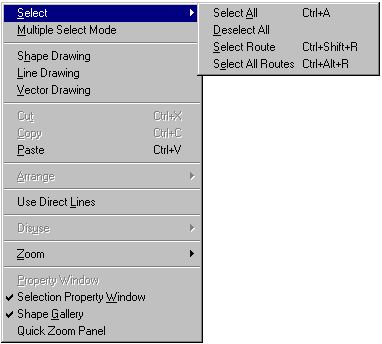
The various WANDA Menus are used to:
quick selection of components to view or edit (see Selection Menu)
compare contents and show differences of two cases (see Compare menu)
choose the desired unit for view/edit (see Units Menu)
specify your other input data (see Model Menu)
view and report the results of your hydraulic model (see Reports Menu).
The diagram short cut menu (right mouse click) gives you fast access to the most important diagram features
At the right side of your screen, the Property Window is displayed.
In this window you can see input and output of a (group of) selected component(s). The Property Window is one of the most important features. It helps you to navigate through your data. The short cut menu (right mouse click) gives you access to the most important property window features.
See for further detail: Property windows.
2.2.2.2. Dialog windows - General
The appearance of all WANDA dialog windows the proceeding is the same, so that the user will get familiar with the program immediately.
All dialog windows contain:
a toolbar
a number of input boxes (white background)
a number of output boxes (blue background)
Toolbar

Most icons are self-explaining (copy, past, save, open, etc.). Read the tool tip to understand the feature.
Input, Output and Units
We would like to draw attention on the following three buttons in the toolbar:
 Displays the input of a selected component
 Displays the output of a selected component
 Displays the possible units for a selected property of a selected component.
Input boxes
For all characteristics, default values are supplied. If an input box is grey, no values can be entered. The values in the white boxes can be edited.
Output boxes
For all type of components calculated output values are displayed in boxes with a blue background. These values cannot be edited (read only).
2.2.2.3. Tooltips
ToolTips are short messages that appear in bubble text. These messages help to explain the name of the tool or button and, in some cases, what the tool or button does.
In WANDA all functions, buttons, icons, etc. have their own ToolTip. It is advisable to look at these tooltips first before selecting a WANDA 4 option.
2.2.3. WANDA 4 in 10 steps
2.2.3.1. Step 1. Add Components
2.2.3.2. Step 2. Connect Components
2.2.3.3. Step 3. Set Component properties
2.2.3.4. Step 4. Set other inputs
2.2.3.5. Step 5. Use advanced features
2.2.3.6. Step 6. Calculate steady state
2.2.3.7. Step 7. Specify hydraulic actions
2.2.3.8. Step 8. Calculate transient
2.2.3.9. Step 9. View output
2.2.3.10. Step 10. Report results
2.3. Building the diagram
For the diagram the incorporated program iGrafx Flowcharter is used. All features about diagram editing is explained in the separate Flowcharter Manual and Flowcharter Online Help.
In this chapter the WANDA related topics are explained.
2.3.1. Shape Library / Gallery
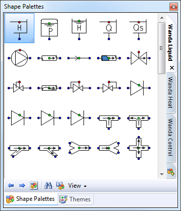
The default shape Libraries WANDA 4 shows are:
WANDA Liquid
WANDA Heat
WANDA Control
In the future new galleries will be introduced for other physical domains or hybrid components. Special made components for particular clients are stored in the “WANDA special” gallery.
To show the status of some active components, like PUMP and VALVE, WANDA uses a extra gallery “WANDA Dynamic” but this gallery will be hidden.
It is possible to assemble your own gallery which contains a subset of the standard galleries. This can be easy to use only one gallery with the frequent used components.
To create your own gallery, consult the iGrafx Help (Shape pallet, F9 – Media manager)
If the gallery is not visible, go to menu view /show gallery or click right in the diagram to activate short cut menu and check Gallery.
By dragging the components in the library you can change their order, or edit the size of the icons.
Default only the shape is visible in the gallery. The tooltip informs you about the particular type. To display this type in the gallery, use the right mouse menu
2.3.2. Adding components
You can add components in the diagram by selecting them in the gallery and dragging them into the Drawing Area.
For details on this subject we also refer to the iGrafx Flowcharter Help.
Each component gets automatically a name starting with the first character of the component type followed by a sequence number. This name can be changed in the property window. The combination “Component type + local Name” must be unique.
2.3.3. Looking closer at components in the diagram
When we take a closer look at the components we see that they have several connect points in different colours. We distinguish physical connect points and control connect points. The physical connect points are used to connect other components which belong to the same physical domain. Therefore each domain has his own connect point colour: blue the Liquid domain, and orange for the heat domain.
It is not possible to connect different coloured connect points to each other
The red and green connect points are reserved for the control module
Note that the shape of a component indicates the positive flow direction if applicable (e.g. P1 and V1 in the picture above). You can change the flow direction by flipping or rotating the component in the Arrange Menu.
For details on this subject we also refer to the iGrafx Flowcharter Help.
2.3.4. Connecting components
Connecting components is as simple as adding them. All you’ve got to do is select a component and drag the mouse pointer to another component.
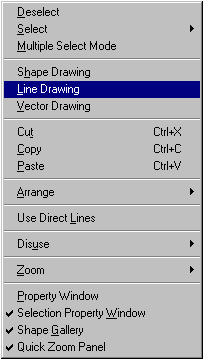
To switch to line mode, activate the right mouse click menu and choose “Line drawing mode”
You can also use the Connector Line Tool  from the Toolbox, left of the Diagram.
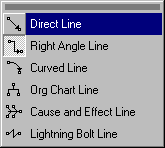
For WANDA 4 diagrams, it is recommended to use only the first three types from the menu below.
See also iGrafx Flowcharter Help for details on drawing and manipulating connections.
2.3.4.1. Master and Slave connections
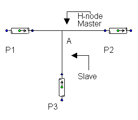
The H-node is represented by at least one single (master) connection line that can connect none, one or two H-components. With extra slave lines it’s possible to connect more than two H-components to one H-node
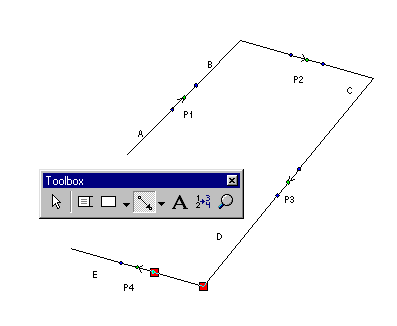
A connection line that is NOT connected to any other line is called a master line. The first connection line you draw is always a master line. Slave lines are connected by ONE end to another master or other slave line. It is not allowed to draw a line between two other lines.
If you select a connection line both ends are marked with a square. The colour of this square is very important. When the square is red it tells you that the line is connected to another line or component. If the square is black the line end is connected to nothing. It’s possible that a line is visually connected but is not connected for Wanda. In this case you see a black square at the fake connected end of the line. When you press the pause button while the property window is active you can see the connectivity of h-components and h-nodes used by Wanda.
The easiest way to fully understand connections is to draw some arbitrary connection lines. If you draw something that is not allowed (schematically) Wanda popup a message and deletes the illegal lines”.
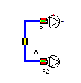
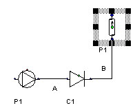
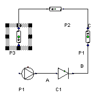
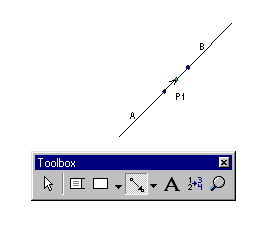
Step 1. Adding connection A (master) between P1 and P2
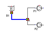
Step 2. Adding connection (slave) from B1 on to connection A
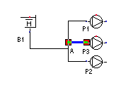
Step 3. Adding connection (slave) from P3 on to connection A
The pictures above show the steps to create a “complex” H-node.
The master and the slave connection line belong to the same H-node. So it doesn’t matter which line you select to edit the properties.
Strings of lines
If you want to connect two components over a long distance it is easier to draw the connection with several shorter lines
First draw the master line that is connected to none or one H-component. Than draw a slave line from the free line end to a second (grid) point. You can attach a second slave line from the free end of the first slave line (and so on).
Deleting master lines
If a line is deleted automatically all lines attached to this line are also deleted. If you do not want this, disconnect the attached lines before delete.
Combining / splitting H-nodes
When one end of a master line is connected to another line, the master line is automatically converted to a slave line. When you disconnect a slave line from another line it is automatically converted to a master line.
2.3.5. Rules for creating a hydraulic model
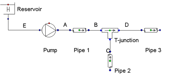
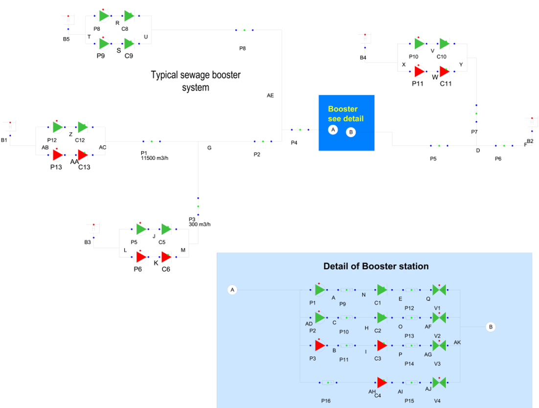
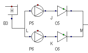
A hydraulic model usually consists of several H-components of different classes connected in a specific way. An example of a hydraulic model is given below.
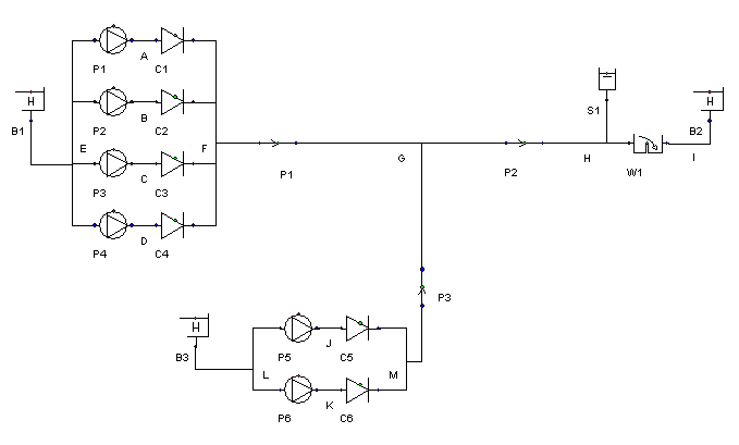
A hydraulic model is built according to a few simple rules. If possible each rule is validated directly and in case of incorrectness a message explains the violation.
Rule 1
A fall-type component has two hydraulic connections: a “FROM” connect point (1) and a “TO” connect point (2) (also called the left-hand side (lhs) and right hand side (rhs)).
The relative position of the two connect points also defines the positive flow direction through the component. This direction is from left to right (FROM –> TO).
Rule 2
A supplier has 1 hydraulic connect point (the FROM).
Note that the positive flow direction at the supplier is from the supplier to the attached H-node.
Rule 3
The number of BOUNDH H-components in the model must be at least one; the number of BOUNDH H-components connected to one connection should be no more than one.
Rule 4
A hydraulic connect point has only 1 incoming or outgoing connection line
A good hydraulic model must be valid (satisfying the four rules above), consistent with the actual piping system and readable. The readability helps to check the consistency of a hydraulic model. For complex systems, however, symbols and straight lines are readily entangled, which makes the model confusing.
As a final remark, it should be noted that building a hydraulic model is by no means a simple “translation” of a real piping system into a computer model following the above-mentioned rules. The rules introduced in this section serve only as a guide for building such a model. Practical skills and engineering judgement are necessary when making a hydraulic model. For example, many details of a real system are actually unimportant for the flow process simulated and can therefore be omitted in the model. This not only saves labour and computer time, but is sometimes also necessary when the system is large and the computer capacities are limited.
An experienced user of WANDA, combined with adequate practical skills and engineering judgement, will find in WANDA a most useful and powerful tool for solving various problems related to transient flow in complex network systems.
2.3.6. Advanced drawing a scheme
It is not necessary to place the shape one by one in the diagram and after that to made a connection between them. You can do it in one simple action.
Select the required component from the shape gallery and move the mouse to the existing component. The mouse cursor changes into the connect icon. Now, drag the mouse to the required location and release the button. The program will determine the direction of the new component based on the position of the connected component.
The scheme below has been drawn using the drag and drop feature, and not using flip or rotate.
2.3.7. Vector based schematisation
The default way to create your scheme is point based: the component is placed in the diagram as defined in the gallery. For GIS oriented diagrams you have to rotate this component. This may be a lot of work.
There is a way to draw the diagram vector based.
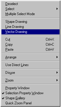
First select the component at the shape library you want to draw as vector. Switch on to Vector drawing mode, using the short cut menu.
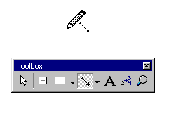
The mouse cursor is changed to a pencil with a line symbol.
Now you can draw the line. The component selected in the shape library is now automatically inserted in the middle of the new line. The component is automatically rotated to the direction of the line. Click in the shape gallery to select another component. Switch of the vector drawing mode when you are finished.
PS: If the component is a supplier it is attached to a free end of the new line.
2.3.8. Aligning routes
WANDA 4 offers the possibility to align certain routes or parts of it. This can be useful, e.g. to match the diagram with the actual geographical situation.
See for further detail the Arrange Menu.
2.3.9. Changing the flow definition
The direction of the positive flow is depicted in the H-component symbol. The sign of the calculated quantity corresponds with this direction.
If you want to change the positive flow definition, you have to “flip” or rotate the symbol.
Use the menu option Arrange/Flip positive flow direction” to reverse the symbol or the short cut menu.
See for further detail the Arrange Menu.
2.3.10. Navigating large diagrams
If the diagram contains a lot of components, it will be quite difficult to fit them in one screen in a readable way. If you increase the zoom factor you have to scroll using the horizontal and vertical scroll bars. You lose the overview about the screen.
This can be solved using the quick zoom panel. Choose “Quick Zoom” from the View menu.
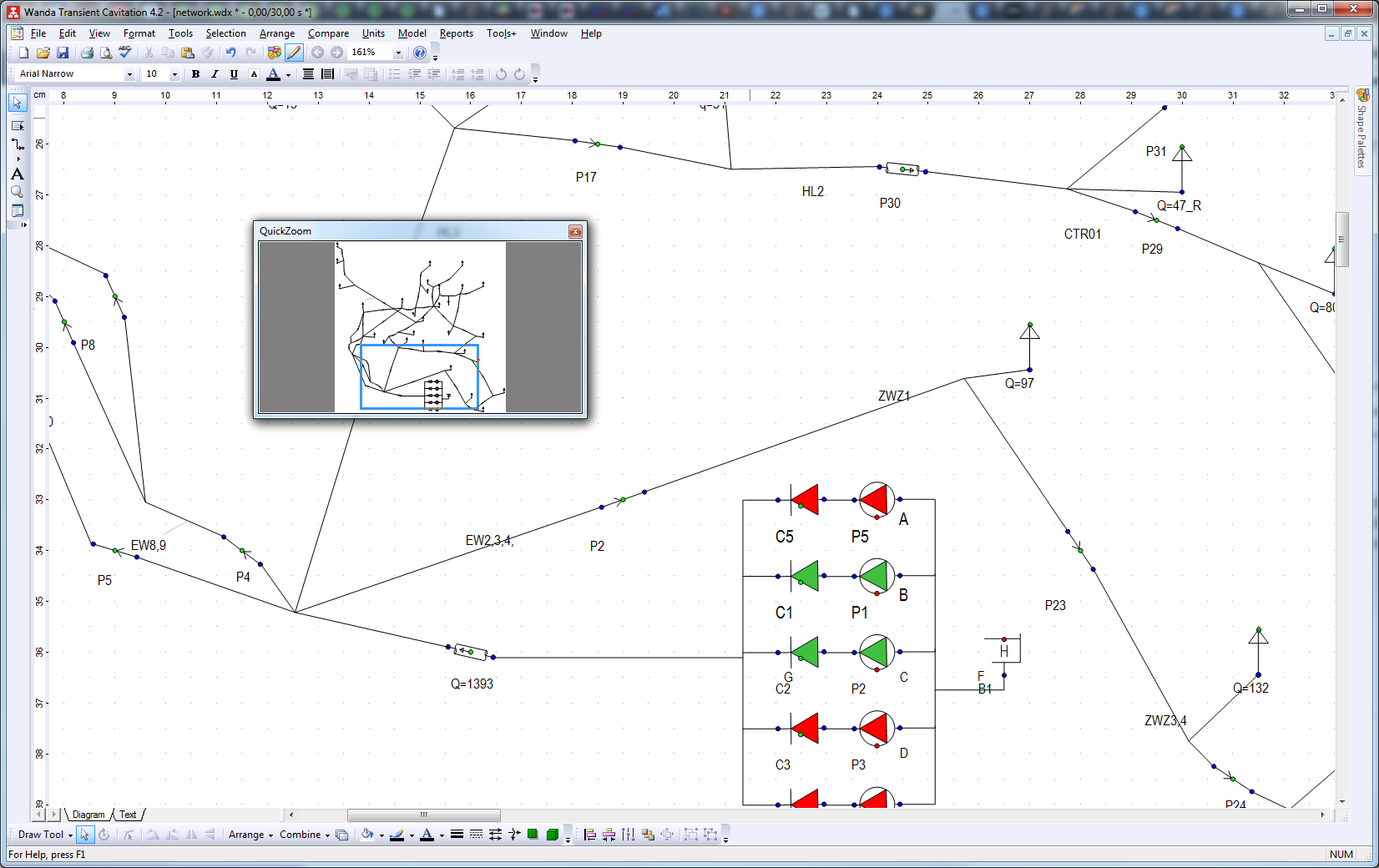
A New dialog will appear. The whole system is displayed in the new Quick Zoom panel. Select in this part a component and the focus of the main window is automatically re-positioned. The zoom factor of the main window can still be adjusted.
2.3.11. Splitting a diagram
To enhance readability of a complex diagram one can use sub-diagrams. A connection line can be split in two using connectors as indicated in the figure below.
To split the selected master connection line go to “Line and Border” in the Format menu. In the “Format Line” windows select the tab “Arrows and Crossovers”. In the corner left below select the checkbox Connectors. The line is split using connectors with a ‘gap’ in between.
Slave connection lines formerly connecting to the split master line should probably be relocated as they now appear to float freely in the gap between the connectors.
2.4. Property Window
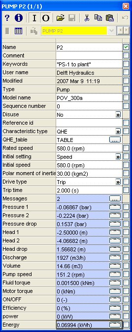
2.4.1. Properties of a Component
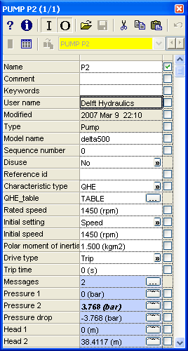
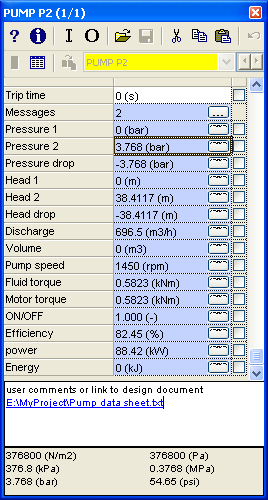
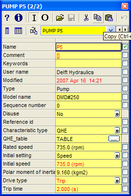
A hydraulic component has several kinds of input and output properties (see Help on Overview of Liquid components). For editing the input properties and viewing the output properties we use the so-called property window.
The Property window applies to individual and groups of selected components. See also: How to use Property Windows.
You see an example of all input and output values of PUMP P1 below.
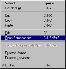
The property window has his own context sensitive short cut menu which gives you access to common used acts.
2.4.2. Visibility of properties
The content of the property window is for each component different.
See also
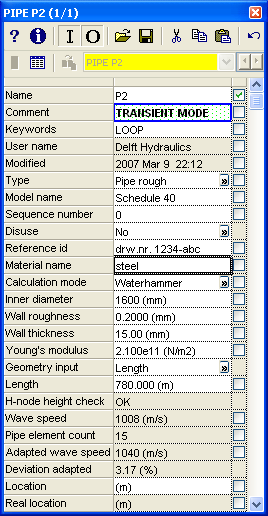
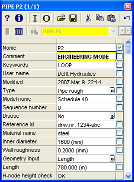
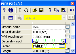
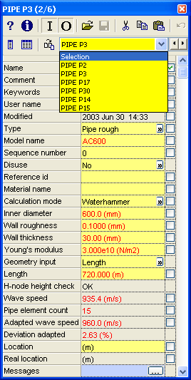
The content of the Property Window depends on the operation mode or input values of other properties. An example of mode dependent properties is the component PIPE. In Engineering mode only the length, diameter and wall roughness are required and must be specified; other properties are hidden. In Transient mode the Young’s modulus and wall thickness must be specified in addition. These dependencies reduce the user input to the required minimum number of properties.
The following examples show the Pipe input properties for engineering mode and transient mode:
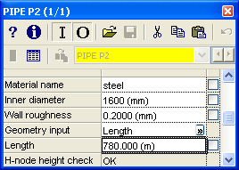
The contents of the Property Window may also depend on the value of a particular property. As an example the geometry must be specified for the Pipe. The geometry may be specified in several ways: by means of the length, a longitudinal profile or a 3D-geometry. The type of geometry is specified using a list box. The appearance of the Property Window depends on the choice in the listbox ‘Geometry input’. See examples below.
2.4.3. How to use Property Windows
The Property Window is one of the most important features in WANDA 4. With this feature it is very easy to view the characteristics of one or more components.
It enables the user to view these characteristics
individually or
in relation to other selected components.
When you select components in your model, its properties and values are automatically displayed in the Property Window. Therefore it is recommended to keep it always open. In this way you can see model, components and properties at a glance.
2.4.4. Example
2.4.4.1. Individual components
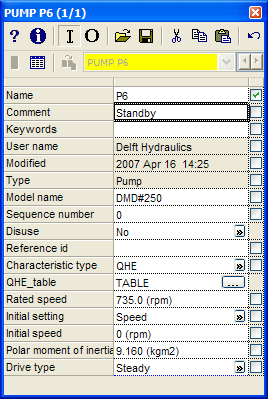
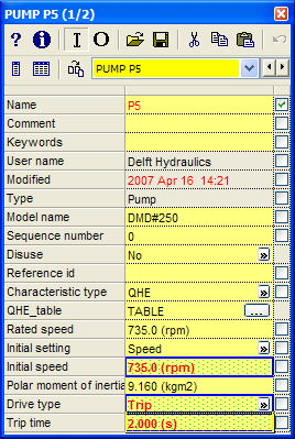
If you select pumps P5 and P6 in the model then the property values for P5 and P6 (individual) are listed in the Property Window:
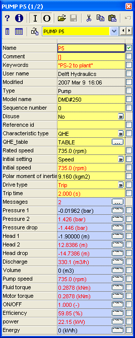
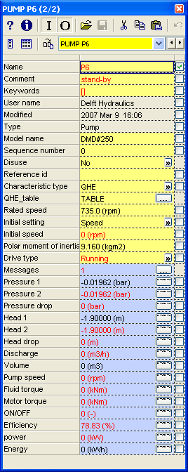
Inputs and Outputs of P5 and P6 are displayed in the two Property Windows above. The caption shows which component is on top. This is indicated in the diagram by a red circle.
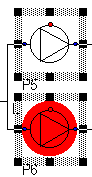
In this way you know at which component you are looking.
2.4.4.2. Font Colours
The colours used in the property window have a special meaning.
Values in black-coloured text are identical for the selected components. The edit field ”Type” is the same for both valves for instance.
Values in italic font are linked to extra information. In this example some information is linked to the field “Inner diameter”. For more information on the linking of extra information see “Toolbars” below.
Values in red-coloured text are different for the selected components. Name and Initial setting for V4 and V7 differ from each other.
Values in blue-coloured text are selected or edited. You can (de)select values using the space bar, dragging the mouse in the input area or click in the description area.
Properties with a yellow background are editable properties.
Properties with a grey background are read-only inputs and can’t be modified.
Properties with a lilac background are read-only outputs (calculated) and can’t be modified.
If the output properties have an orange background and a strike-through font, this means that one or more properties in the model are changed and the output is no longer valid anymore. The results are still accessible until you close the changed case.
2.4.4.3. Toolbar
The buttons in the Toolbar enables you to display the desired information by toggling on or off the buttons and to manage the data in an efficient manner.
All buttons are explained below:
 /
/  Help
Help
Toggling on Help (or key F1) shows the Wanda Help relevant to the active component. With Shift+F1 the user can add a so-called user-defined help entry in a WordPad file. The question mark gets a yellow background to show that a user defined help entry has been made. In this way the user can extend the standard WANDA Help. It offers the possibility to add tips or tricks related to this component. If the file is saved on a network drive, all other WANDA users in the company can access this information.
 Information
Toggling on Information shows two extra information fields. One field that shows what units can be used for this property (see also Units Menu). In this example it shows the available diameter units:
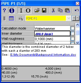
Furthermore, it shows a field with additional information on the selected property. In this case it shows how the Inner diameter of this pipe is calculated: You can also put links to Word-documents or other files in this extra information window. Even pictures are possible. Properties with additional comments can be recognised by a different font (bold+italic). All additional information is saved in the Wanda wdi-file.
Click the right mouse button, for an additional edit menu, to modify your comment:
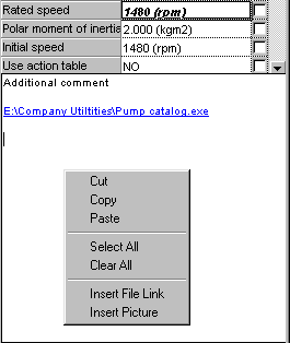
This comment feature is very powerful for quality assurance at project level. Now it is possible to add essential information to each component property. This linked information allows easy access for project reviews, (external) audits, and simple follow-up of projects by colleagues.
 Show/Hide Input
This button shows or hides the input properties of the selected component.
 Show/Hide Output
This button shows or hides the output properties of the selected component.
 Property Template File Management
Open a property template file and apply it to this component, if relevant (see also: Creating your own database system). The retrieved data are displayed in blue.
 Edit
Edit
These buttons enable you to:
Cut the selected (blue) values to the clipboard
Copy the selected (blue) values to the clipboard
Paste the content of the clipboard in this window and thus use it for this component, if applicable (see also: Editing or Synchronising values).
 Range View
Activating this button shows an overview of the value ranges of all properties of all selected components. This is useful for inspecting the hydraulic model.
 Spreadsheet View
Activating this button shows a tabular view of all selected properties of all selected components. This is useful for inspecting and editing into this selection.
 Copy / Synchronise
This button enables you to Copy (synchronise) the blue-coloured properties to the selected objects in the diagram. See Editing or Synchronising values.
Checkboxes and buttons
Check boxes on the right of the Property Window are used to display or hide the value in the diagram. Component names are displayed by default. You can add other relevant properties to your diagram by checking the boxes. The displayed info remains correct because of the link between the Property Window and the diagram. The property values are put in a text box in the text layer.
For an explanation of the buttons in the edit and output fields, see:
 (Use Table): see Tables and tabular views,
 (Show Graph): see How to use charts.
2.4.4.4. A group of components
The Property window enables you also to see significant values for a group of selected components, by choosing ‘Selection’ in the drop down menu below the toolbar:
After choosing ‘Selection’ you see the properties in the selection of the components (read-only). If values differ the range of values is shown.
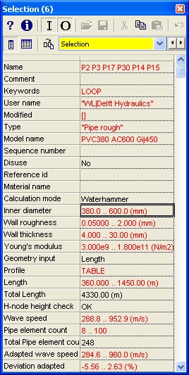
In this example only two components of the same type are shown. Therefore the selection of values is rather transparent. The situation is more complex, if you select more components of various types.
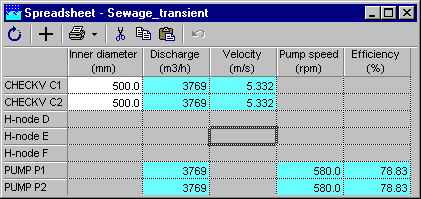
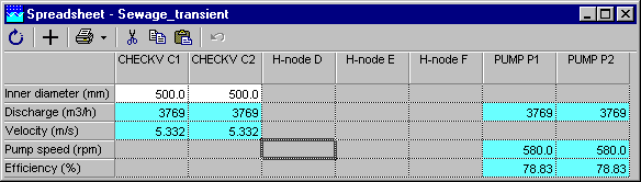
2.4.4.5. Spreadsheet
With a spreadsheet you can edit multiple properties of multiple components/nodes.
You can copy easily copy/paste selections to Excel/Word.
You can create a spreadsheet by pressing the “grid” button at the Property Window.
You get a view with the selected objects in the diagram and the selected properties in the Property window.
To rotate the spreadsheet press the left button; columns and rows will be exchanged.
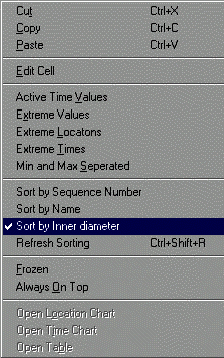
The spreadsheet has his own context sensitive short cut menu. For example, this menu can be used to sort the spreadsheet on an arbitrary column, the selection sequence or a user–defined sequence.
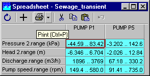
Output ranges, including the corresponding time and location can be viewed in an easy way. The contents of the spreadsheet can be frozen during the edit and simulation session to compare the results with other calculation made within the same session
The tabular view is automatically updated when input or output is changed. When the selection of objects and properties is changed, an existing tabular view keeps unchanged. You can create multiple spreadsheets with different selections.
With the drop down list near the print button, you can set up and create print reports of the spreadsheet.
2.4.4.6. Editing or Synchronising values
As discussed the Property Window is the feature to have a detailed look at the components in your model. You can see differences between components immediately, indicated by red text.
Sometimes these differences are unintended. The Synchronise (or copy) feature allows you to solve this problem.
In the property window above you see the properties of pump P5, in a selection with another pump P6. You can see that the (red-coloured) values for the properties differ from P6.
To synchronise one or more altered values for both pumps, you only have to select the values you want to synchronise. To select, drag the mouse or press the space button. Bold text together with a dithered background and a blue outline, indicates which properties have been selected.
When you click  (or shortcut key Ctrl+Enter) the selected values are copied to pump P6.
Note that the output has disappeared from the Property Window after applying Synchronise. The output has to be recalculated, due to a change in input parameters.
2.4.4.7. Tables
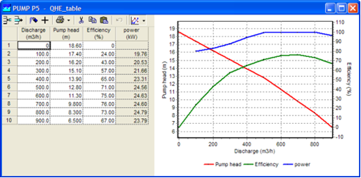
Pressing opens a table. Some properties, like pump characteristics, pipe profile or action table, are non-scalars but multi-column data series.
The table displays 2 or more input columns. In case of a pump, a read-only column shows you a derived quantity. The edit grid acts as a spreadsheet.
Some type of tables must satisfies certain rules, e.g. a pump capacity curve (QH) is monotonously decreasing; values in first column must be in successive order. If the input doesn’t satisfy the rule the colour becomes red.
Taskbar
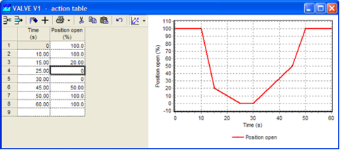
The first two toolbar buttons above, allow you to insert or delete rows in the action table
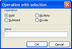
The ‘plus’ button activates a new window to carry out some simple numerical operations at the selected cells.
‘Auto fill’ can be used to fill empty cells between two values, using linear interpolation.
The button on the right displays a graph of the table.
See: How to use charts.
Example of pump characteristic table:
Example of Valve action table
2.5. Selection Builder
2.5.1. How to use the Selection Builder
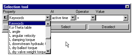
In WANDA 4 it is very easy to select single (or groups of) elements. A tool that is very helpful is the Selection Builder (accessed via menu Selection/Selection Builder Window) With this tool you find elements, selected on:
Properties (input and output properties)
At a given time step or during all calculated time steps
Applying a certain operator ( =, <, >, <>, like)
With a given value for the properties.
In this way you can select elements by keywords, inputs and/or outputs. Keywords can apply to any selection (see Add to/ Remove keyword from selection…). You can even build complex queries by applying the Selection Builder several times in succession and by choosing Select or Deselect.
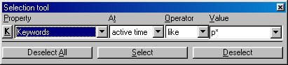
The first 4 operators speak for themselves. The ‘like’ operator is a powerful string-matching operator. The edit field value contains the pattern that is to be matched. This pattern may be a normal keyword, component name etc. Furthermore the pattern may contain one or more of the following special characters:
Character |
Matches |
? |
Any single character |
* |
Zero or more characters |
# |
Single digit (0-9) |
[charlist] |
Any single character in charlist |
[!charlist] |
Any single character not in charlist |
The set of characters in charlist, may contain a hyphen (‘-‘) to specify a range of characters, e.g. [a-k].
Examples
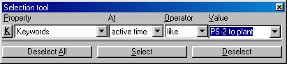
In the screen below we are looking for elements in the model that start with a ‘p’ for the property keyword. (Note that you can use wildcards.)
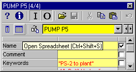
If you want to search on keywords, a dropdown list of available keywords is displayed in the edit value box. We have selected the keyword PS-2 to plant, at the active time, in the example below.
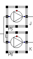
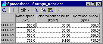
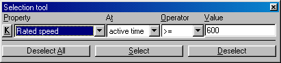
If you want to select all components that have a rated speed of 600 (rpm) or more, you could apply the following selection query. In the diagram, two pumps are now selected.
If you click the ‘K’ button, you will go back to searching by keyword.
TipPressing Alt +F7 activates the Selection Builder.
If you press Alt +F7 while a property is selected in the Property Window, this property will be entered in the Selection Builder.
2.6. Using Charts
2.6.1. Kinds of charts
In WANDA we distinguish three kinds of charts
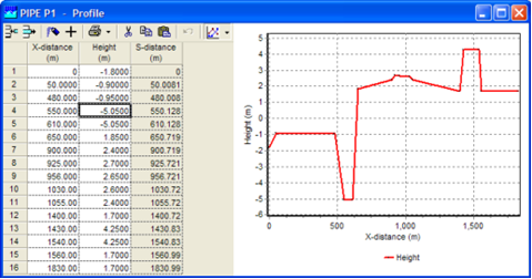
A chart of an input table: (pump curve, pipe profile, action table etc). The quantity and unit of the X-axis and Y-axis depends on the kind of table.
Time series: This chart contains one or more quantities as a function of time (H(t), Q(t), v(t), etc.). See also Time series.
Location series: Output properties of a pipe can be visualised in a chart as a function of the location (P(x), H(x), Q(x), etc). See also Location series for a single pipe.
Each chart type uses its own default chart template. In these templates the layout of the chart is defined. The user may adapt the templates to personal preferences. More information on managing these templates, see Help function of Deltares Graph Server.
2.6.2. How to use charts
If you click the chart button in the Property Window (see How to use Property Windows), a chart of the corresponding output property is displayed. The graph button is part of the output property boxes.
The most important features of charts in WANDA 4 are:
Zoom in on the graph, by drawing a rectangle from left-up to right-down.
Scroll through a zoomed graph by holding the right mouse button.
Change the layout and presentation of the graph by double clicking on the graph or through File menu ‘graph properties’.
Save graph settings in a template, for later use, using the template menu (see also Help Chart server).
Export charts as a Bitmap, Windows Metafile or other formats for use in other applications or documents.
Copy graph data for use in other applications (tab-delimited data, e.g. spreadsheets).
2.6.3. Chart with more series
Each time you click the chart-button a new window is opened. If you want to add a series to an existing graph, just press and drag the button into an existing graph. The series is added to this graph.
WANDA allows multiple documents; that means that another case can be opened and that output of more than one case can be drawn in one chart to compare the results of different cases.
2.6.4. Time series
Time series are applicable in transient mode only!
All output properties of WANDA objects can be visualised in a chart. This chart contains one or more quantities as a function of time (H(t), Q(t), v(t), etc.).
To create a chart with two or more different output properties, for example the upstream pressure P1 and the discharge Q of a valve, first press the chart button of Pressure 1, then drag the chart button of Discharge into the Pressure chart. The result is displayed below.
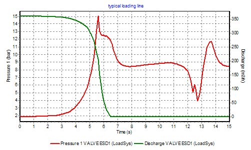
In this way you can also combine different properties of different components.
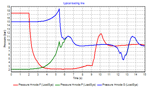
To create a time series chart with two or more time series of the same output property, first select the objects in the diagram, then press the chart button of one of the selected components. The result is that the output property of all selected components is displayed.
To create a time series at a certain location in a pipe, you have to specify a value in the property field “Location”. The program adapts this location to the nearest calculation node, which is shown in the property field “Real location”. If the Location field is empty, pressing the chart button results in a location chart of the pipe. See also Location series for a single pipe.
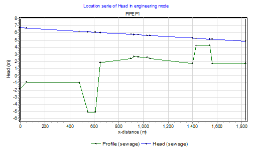
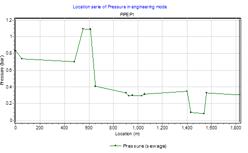
2.6.5. Location series for a single pipe
The representation of the location chart depends on the mode you are running. In engineering mode the entered profile points are displayed as internal points (see below):
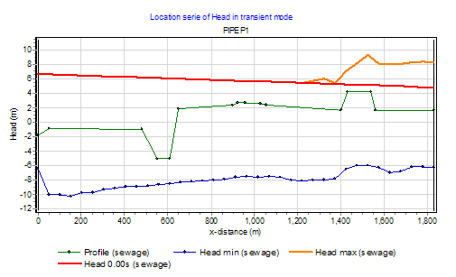
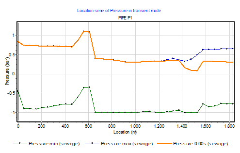
In transient mode the pipe is divided in one or more elements of equal length (based on the wave propagation speed and time step). The output is available in the internal calculation points only (the so-called waterhammer nodes). These waterhammer nodes do not match the profile points. The waterhammer nodes are displayed on the minimum values. The user is strongly recommended to check that the waterhammer nodes cover all relevant high points; decrease the time step if necessary.
In transient mode the chart shows the minimum and maximum values (the envelope) and the values at the current time step. Use the time navigator to analyse the dynamic behaviour (see How to use the Time Navigator). The actual time is displayed in the caption.
The following charts show the same charts as shown in the previous chapter, but now for transient mode:
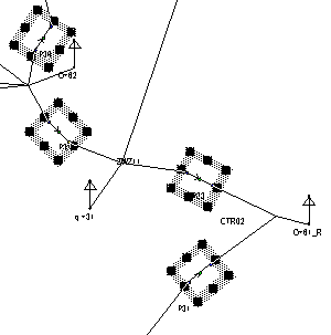
2.6.6. Location series for a route
A route is a sequence (string) of selected hydraulic components without a gap. It is not necessary to select the H-components in a route one by one (extend the selection with Shift+Click). The program automatically selects a route by clicking the first component and Ctrl+Shift+Click the last component. For more information of selecting routes see Diagram routes.
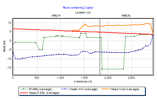
To check if a selection satisfies the route definition, just choose the “Selection” view in the property window (press the A-button). If a chart button is visible at the output properties, the selection defines a route. Only pipe components have a length, other H-components have no length and are not recognised in the chart.
The route function is drawn for the actual time, defined by the Time Navigator (see How to use the Time Navigator. The route creation is the basis for displaying and analysing pressure surge Movies. The actual time is displayed in the caption.
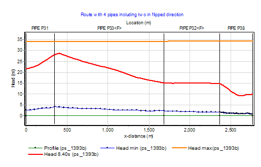
In the chart all pipes are represented in the same flow direction. In a large distribution network it is possible that the positive flow definition is opposite to the current flow. In that case the pipe is represented in flipped position, indicated by a <F>.
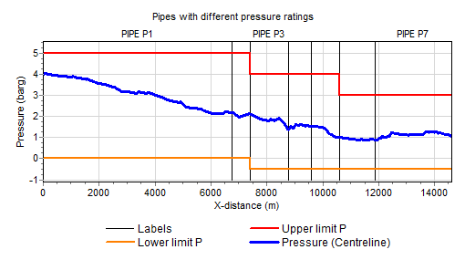
It is possible to display the pressure rating of the pipe in the chart. In the Mode & options menu (Mode and options) a visibility checkbox is available to manage this option. The upper and lower limit values of the pipe are part of the hydraulic input properties of the pipe.
2.6.7. Location axis
For a location series, default the horizontal length is used. The user can switch this horizontal length (X-distance) to the spatial distance (S-distance, real length). Especially for vertical pipe sections this may useful. To change this mode, go to the mode & options menu (see Mode and options).
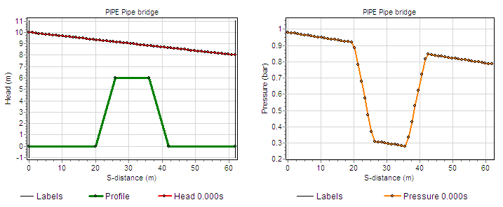
To show the different between both representations the Pressure Head and Pressure charts are given for both axes in case of a pipe bridge (crossing width 10 m, height 6 m).
Bottom axis as X-distance (horizontal):
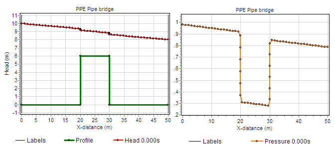
Bottom axis as S-distance (Spatial):
2.6.8. Selection charts
Each time you press the chart button in the property window, a new chart window opens. Without closing these windows your screen becomes full within a few moments. It is possible to open one common chart window for a location and one common chart for a time series. Now, when you select an output value, the series is automatically drawn in the chart window. These so-called selection charts are activated via the context sensitive short cut menu (press right mouse button in the property window).
2.6.9. Chart templates
The layout of the several kinds of charts are defined in the so-called chart templates. These templates are part of the WANDA delivery. The chart template contains the chart properties, which describe the layout of the chart. If you are not satisfied about the layout, you may edit the chart properties. The modification can be stored in the default template or in a user defined template.
To change the chart properties, double click in the chart or use the menu “file”/chart properties”. All changes are applied directly. To store these settings you must save it into a template. Be aware that the axis title, legend and text headers are variable (text depends on case and kind of property). To maintain these variable text items, the template must be saved in design mode. Choose from the Chart menu “Captions/Absolute”. Then save the template via menu “Template/Save” of activate the Template manager.
2.7. Time Navigator
2.7.1. How to use the Time Navigator
The Time Navigator allows you to scroll in time through the calculated results of your model, and look at specific locations and instances in your model.
You can only use the Navigator after you have calculated the model in Transient mode and thus generated output. Activate the time navigator via the menu Model/Time Navigator or press Ctrl+T
By moving the horizontal slider you can see the output (e.g. head or pressure) of a selected component at a selected moment in time. The selected time is visible in the caption of the WANDA window and in the caption of the Time Navigator.
By moving the vertical slider, you can control the speed of the viewed output.
It is also possible to view the output of a component at:
a given time and
a given location.
Example
If we want to see the head for PIPE P1 at t = 11.100s and at location 1500m, we first put the Time navigator at that particular point in time:
After we specify the location in the Property Window of PIPE P1 (see Properties of a Component), WANDA 4 uses the closest calculation point (1525m) as the real location for PIPE P1, which has a total length of 1831m (see pipe length).
2.7.2. Playing Movies
WANDA allows you to play movies of the output of certain components. The transient pressure in a pipe is a wave phenomenon that propagates through the system.
If you want to see the changes in time of a simulation, we first display the graph for the pressure of a certain pipe, by clicking the graph button. The edit field ‘location’ in the Property Window (see Properties of a Component) must be empty in order to view the route consisting of all selected components; see How to use charts for more info on the creation of routes.
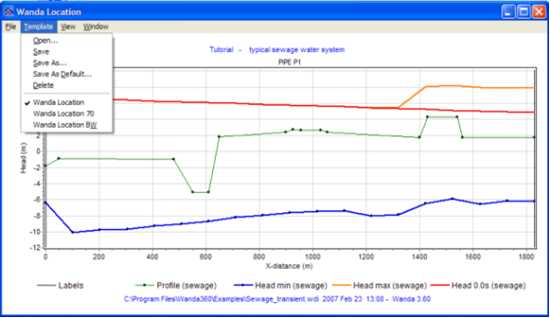
The blue line is the minimum pressure, orange the maximum and red the pressure at a moment in time, along the total length of the pipe (location). The calculation grid is indicated on the minimum series. If the head along the selected pipelines is displayed, then the pipeline profile is displayed as well. The head graph above reflects the dynamic situation after 3.6 s (indicated in the legend).
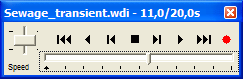
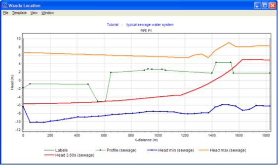
By shifting the time to another moment, the chart shows the new situation automatically:
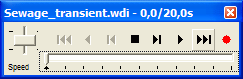
If we click the play button on the Time Navigator the graph will turn into a movie, displaying the pressure in this pipe, in a linear time mode, depending on the simulation time and time steps you have specified for this model (see also Time parameters…). You can view multiple movies in a single graph or in several charts simultaneously, for example movies of the head and flow.
2.7.3. AVI-creator
You can record the movie in a separated file (AVI format) to use it for presentations or to include it in your digital report. The AVI-file can be shown with any media player which support AVI-files.
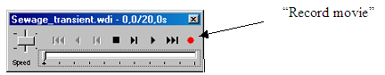
To record the movie, simply press the red record button in the “movie navigation window”. A “Save Dialogue” window will ask for a file name of the AVI –file.
Note that only one location chart window may be active. It is not possible to record two or more location chart windows together.
2.8. Creating your own database system
2.8.1. Property templates
WANDA 4 allows you to create your own set of frequently used settings for all kinds of data. This applies to component properties and specific settings for fluids, accuracy or time parameters.
In this way you can use WANDA 4 the way you want, and adapt the application to your specific use.
Frequently used properties can be stored on disk and re-used. WANDA uses the file system to manage these property templates. An example of such a directory tree is part of the WANDA installation.
For example:
map Fluids contains templates of several kind of fluids
map Pumps contains templates of several kind of pumps
map Pipe sizes contains templates with pipe dimensions for several materials and pressure ranges
map Roughness contains only the roughness property of several kinds of pipe materials.
Important: the delivered property templates are only provided as examples. Deltares not be held responsible for the correctness of the contents.
2.8.1.1. Example: Property window
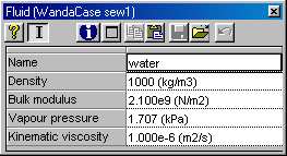
The default fluid window (for Liquid) in WANDA 4, looks like this:
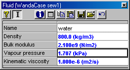
In the model you use, it is possible that you frequently calculate schemes for water of 20 degrees. This means that every time you build a model, you have to adapt the characteristics for water.
In WANDA this problem doesn’t exist because you can create your own template for water of 20 degrees, and store it for later use. All you have to do is give in the characteristics and save them:
When you click the save button, WANDA asks you for a file name:
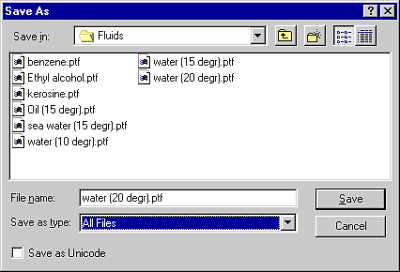
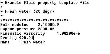
If we open this template in Notepad, it looks like this.
Data is always stored in SI units, but automatically converted if you select another unit system in WANDA.
It is obvious that you can make templates for all kinds of fluids in this way and create your own database system.
The properties are stored in ASCII (text) files with extension “ptf” which stands for Property Template File. We recommend you to extend these files with useful comments.
See next example:
* Source: Catalog Manufacturer XXX
* page II-32a
* Last updated: 1999-09-25 S.O. Mebody Deltares*
Model name HPE 125x110.8
Comment 0.6 MPa SDR176
Material name HPE
Inner diameter 1.108
Wall thickness 0.00710000
Young’s modulus 8.00000e8
If you save component properties to a template, only the selected properties are saved (the blue ones). For the fluid, physical, initial values, user units, all properties shown are saved.
2.9. File Management
2.9.1. File management in WANDA 4
A complete case study using WANDA produces a set of data files, called case files. The case study is identified by a case name, defined by the user. Case files have the same name as case name but differ by extension. File extensions are administrated by WANDA. This section presents the filename conventions and the way to deal with the data files.
2.9.1.1. Conventions for WANDA file names
One set of case files is related to an unique WANDA computation/simulation. To distinguish between different simulations, the user should give a unique case name to each simulation. Case files use the case name as the filename, so that they can be easily identified in the working directory.
The maximum length of a case name including the path (C:…….) is 260 characters (Windows limit). The path and file name may contain blanks.
The general format of filenames is then: “xxxxxxxx.ext” where “xxxxxxxx” is the case name (user dependent), and “.ext” is the extension generated by WANDA. The extensions used, are:
extension |
file type |
wdi |
file for input data |
wdx |
file for iGrafx diagram |
wdo |
file for data generated in both steady and transient computations |
__i |
interface file between the modules STEADY and TRANSIENT |
_sm |
messages (log file) from the module steady-state |
__r |
interface file between the modules TRANSIENT and RESULTS |
_um |
messages (log file) from the module transient-state |
wir |
ascii file containing the input report |
wor |
ascii file containing the output report |
wps |
ascii input file used for parameter run |
wcr |
ascii output file with case compare results |
rtf |
log file, written by closure of case file |
csv |
ascii output file (column separated) with summary output parameter run |
wdd |
ascii file containing the case description text; handy for preview in a file manager |
wmf |
file containing the diagram picture; handy for preview in a file manager |
It is recommended to choose a case name, which contains as much information about the system and process simulated as possible. One may think of, for example, “oilload” or “pumptrip”.
One often needs to make several simulations based on the same hydraulic model. This is possible provided that each simulation has a unique case name. It is advised to administrate the simulations by having serial integer numbers included in the case name, for examples, “pumptrip01”, “pumptrip02”, etc.
2.9.1.2. Important files for backup
For backup purposes it is recommended to store at least the WANDA input files in a save place. It is not necessay to store all files because the output files can be generated easily again.
To store the complete input, you need only the “wdi” and “wdx: file.
2.9.2. The File Menu
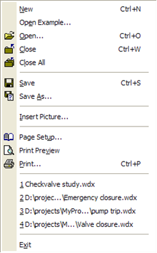
The WANDA File Menu has, next to the traditional, menu options, a few specific ones (see for details Help on iGrafx Professional).
If you choose:
New: WANDA 4 opens a file called Untitled.wdx. In the caption you also see “(no output)”.
Open: opens *.wdi-files
Save as: saves *.wdi-files
Close: When closing, WANDA 4 asks “Save changes to *.wdx?”
At the bottom of the menu you see projects and files, that were used in previous sessions.
Note: You can open and view diagrams, inputs and results of all kinds of WANDA cases in WANDA 4, including cases that contain components that are not covered in your license agreement. You can not save cases that are not covered by your license agreement; the Save and Save as…. items are disabled.
2.9.2.1. EPANET / ALEID import
WANDA supports the import of EPANET and ALEID models. ALEID is a Dutch program used for drinkwater distribution (based on Epanet scheme).
To import an EPANET or ALEID model, choose from the file menu “Open” and select from “Files of Type” EPANET project (.inp) or ALEID project (.pro).
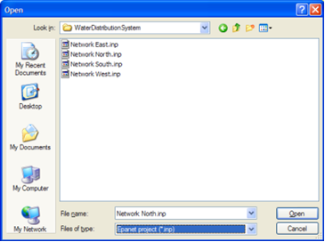
From the distribution model, the next data is converted: pipe length, pipe diameter, wall roughness, H-node elevations, delivery rate (H-component TAP).
Converting these files takes some time dependant of the network size. Be aware that the network size match your WANDA size license.
2.10. Arrange Menu
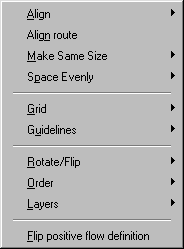
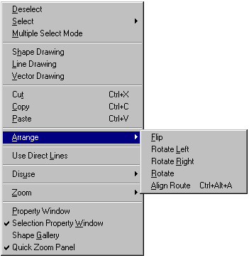
The Arrange Menu allows you to edit the layout of the diagram. Most features are also accessible using the context sensitive right mouse click menu.
In addition to the iGrafx Arrange Menu, WANDA 4 offers two additional features, especially for use in Hydraulic schemes.
2.10.1. Align route
Aligns a selected route between several hydraulic components, for the purpose of reporting.
Note: When aligning routes it is important that you have used direct connection lines.
The pictures below show how to align a route of components:
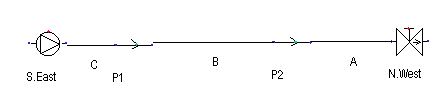
Schematic situation: A flow from South East to North West
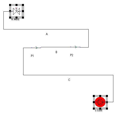
Real situation: North West (top-left), South East (bottom-right)
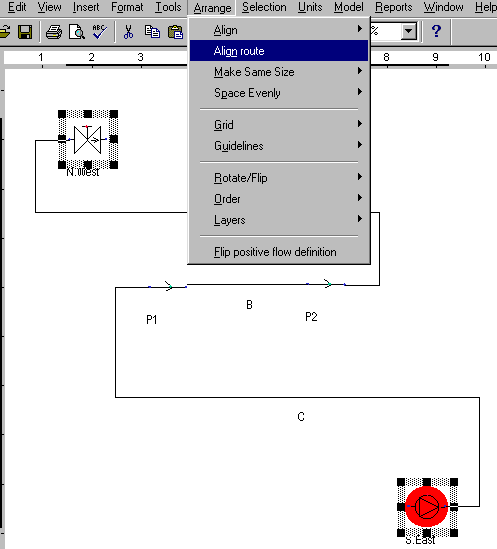
Aligning real situation
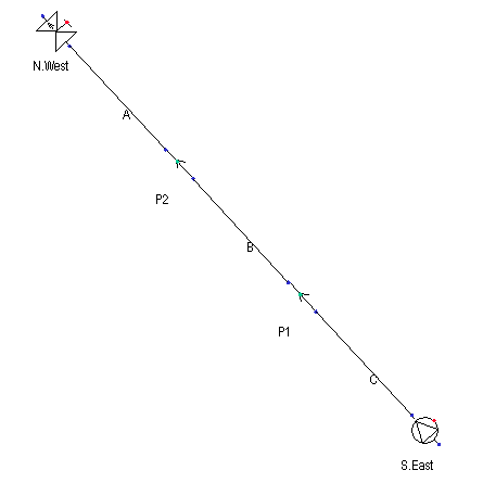
Result
Tip: It is also possible to draw a series of components in a particular direction using the Vector based schematisation.
2.10.2. Flip positive flow definition
Allows you to change the flow direction (definition) of selected components.
The pictures below give an example:
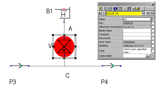
Valve V5: flow direction from A to C. Note the property ‘Attached Connections’ in the Property Window.
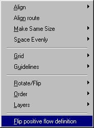
Choosing ‘Flip positive flow definition’ in the Arrange Menu
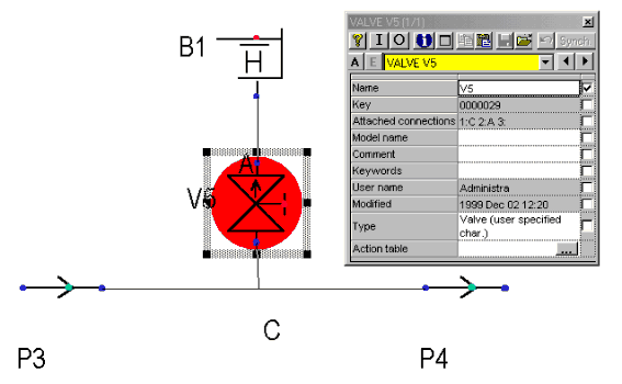
The Flow definition of Valve V5 is flipped (see also Attached Connection)
The flip feature is also supported by the flip button in the draw toolbar.
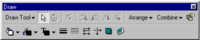
If the draw toolbar is not visible, select Menu/View/Toolbars.
2.11. Selection Menu
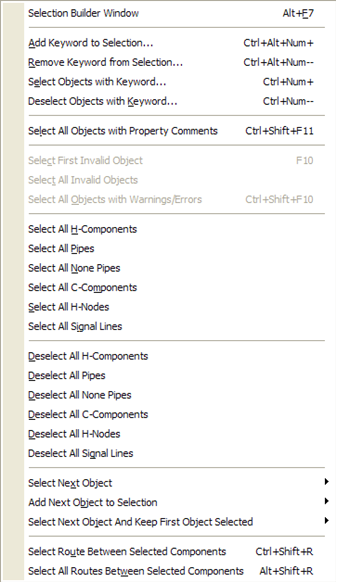
In the Selection Menu you can view and edit all kinds of characteristics of components in your model, by simply selecting one, a group or all the components.
See also: Selection builder.
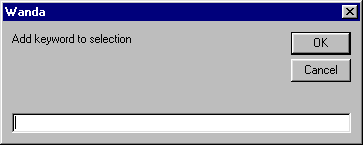
2.11.1. Add to/ Remove keyword from selection…
WANDA 4 offers you the possibility to shape and build the hydraulic model to your preferences.
Each H-component and H-node has a keyword property. This is a text string up to 50 characters. The string may contain more than one keyword. Use quotes (e.g. “from A to B”) if the keyword contains spaces.
Keywords are used to select a certain group of objects with a special meaning, e.g. a pump station, a network extension, a route etc. This means that an object can contain more than one keyword. To add or remove a keyword from a selection you need this feature.
Note: if you use the synchronise button in the property window, each object gets the same keyword(s). Now only the specified one is added/removed.
In this way it is easy to find a group of selected elements, by using the Selection builder.
2.11.2. Select invalid components
In some cases the calculation of your model is not performed. This means that one (or more) component(s) in the model are invalid. They can be of the wrong type, in the wrong place or may have the wrong input. All these faults depend of course on the type of model you want to calculate.
In the selection menu it is possible to select these invalid components by choosing:
Select first invalid component: selects first invalid component in the flow (press F10)
Select all invalid components.
If there are no invalid components this option is grey and cannot be used.
2.11.3. Select components and/or connections
The function of these options is self-explanatory.
It is advisable not to select an element before using one of the options. E.g. if you have selected all pipes, and afterwards you select all connections the selected pipes will stay in the total selection.
It is possible to select:
all H-components
all pipes
all none pipes
all H-nodes
all C-components
all signal lines
2.11.4. Deselect components and/or connections
This function is the opposite of Select components and/or connections and therefore self-explanatory.
Note that you can use both features in addition to each other. You can for instance select all H-components and delete all pipes form this selection by using ‘deselect all pipes’.
2.11.5. Select route between selected components
When you have selected two components, this feature selects all components and connections (H-nodes) on the shortest route between the two selected components.
In this way you can easily compare or synchronise certain components or store the selected route under a keyword.
It is now possible to look specifically at the output of the selected route. When the graph button is displayed in the Property Window (focussed on selection – press ‘A’) you have created a valid route.
The pictures below show how to select a route:
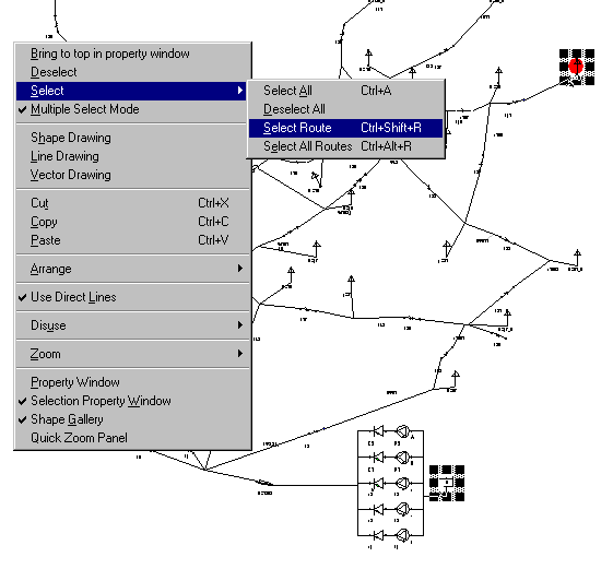
Two components in the model are selected. By choosing “Route between selected components “from the Selection Menu all components along the route are selected.
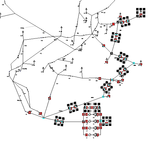
All components along the route are selected in the diagram.
A very fast way to select a route is done by a combination of mouse and keyboard.
First click (select) the beginning of the route, then click the end of the route with the Shift key pressed down.
The select route option is also accessible via the right mouse click menu.
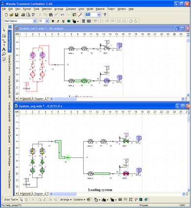
2.12. Compare menu
The compare menu allows the user to compare two cases that are opened simultaneously. If more than two cases are opened, this menu cannot be used. In this way the user can easily find which objects are changed, and which objects are added. This can be very useful in a study trajectory, in which more than one version of the model may be created.
Below the Compare menu is shown:
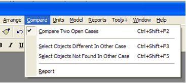
Comparison is primary based on the unique key each object has (like H-component, H-node, C-component, signal line). This key is normally hidden but can made visible by pressing the pause key with the property window active. The graphical location in the diagram is not taken into account during the comparison, neither other graphical attributes.
Checking the “Compare Two Open Cases” marks all objects with different input properties with a coloured hatch. Differences in property values itself (input and output) are marked in red.
2.12.1. Objects different in other case
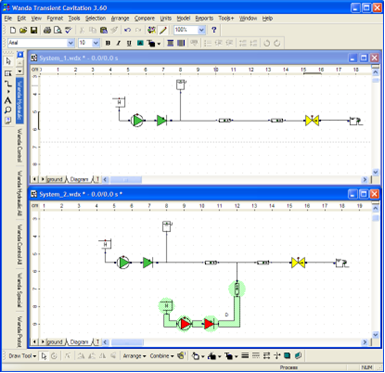
When we compare System_1a with System_1b, an object is highlighted with blue hatches. In this situation the key of the object is equal for both cases, but its properties are not. E.g., in the case shown in figure below, the length of the pipe is 1000 m for System_1a and 1200 m for System_1b
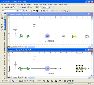
When selecting the object, the property that is different is shown in red in the property window. If we move the mouse to this value, the value of this property for both cases is shown in a light yellow box, see figure 2 in which we have selected the pipe from System_1a: the pipe length of System_1a is printed in front of the ‘<>’ and the pipe length of System_1b after the ‘<>’. Note that every input property that the user can change, may trigger that an object is found which is different in the other case, although the hydraulic behaviour may be identical (i.e. when adding some comments, or changing the name of an object).
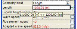
2.12.2. Objects not found in other case
When we compare System_2 with System_1, using ‘Compare Two Open Cases’ (Ctrl+Shift+F2), some objects are highlighted with green hatches, see figure below. This is because these objects do only exists in System_2 and not in System_1. Here we note that Wanda uses only the key of the components when it is looking for objects that do not exist in both cases.
With the compare menu it is also possible to select all objects that are non-existent in the other case (highlighted green): Ctrl+Shift+F5, or to select all objects that are different in the other case (highlighted blue): Ctrl+Shift+F3.
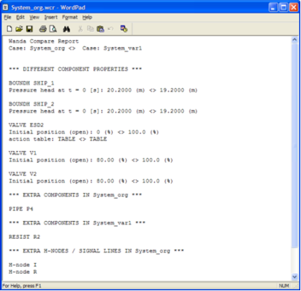
With the option report, a report is printed on screen and saved as a wcr-file.
See example below
2.13. Units Menu
2.13.1. The Units Menu
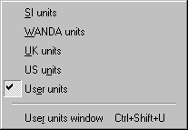
Several unit systems are supported in WANDA. The user can choose among the following systems:
SI units (SI) (System International)
WANDA units (WD)
Imperial units UK)
ANSI units (US)
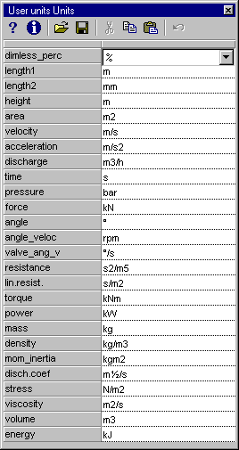
User units (User)
Default units are user units. The user unit table can be configured with your own preferences.
The selected unit system is used for the input and output of data. However, WANDA uses the SI units as the internal system. Conversion between the internal unit system and the system selected by the user is made automatically via the built-in system interface. The user is completely shielded from the internal unit system.
Within a WANDA session with multiple cases active, there is only one unit table active. The last opened case defines the actual unit system, which is used for all open cases.
Next tables shows the contents of the available unit groups and the conversion factor used.
The factor is defined as:
value [user units] = value [SI-units] * factor.
Dimension |
SI |
WD |
UK |
US |
User *) |
dimless |
‑ |
‑ |
‑ |
‑ |
‑ |
length1 |
m |
m |
ft |
ft |
m |
length2 |
m |
mm |
inch |
inch |
mm |
height |
m |
m |
ft |
ft |
m |
area |
m2 |
m2 |
ft2 |
ft2 |
m2 |
velocity |
m/s |
m/s |
ft/s |
ft/s |
m/s |
acceleration |
m/s2 |
m/s2 |
ft/s2 |
ft/s2 |
m/s2 |
discharge |
m3/s |
m3/h |
gpm |
gpm(US) |
m3/s |
time |
s |
s |
s |
s |
s |
pressure |
N/m2 |
kPa |
psi |
psi |
barg |
pressure_abs |
N/m2..a |
kPa.a |
psi.a |
psi.a |
bar.a |
pressure_drop |
N/m2 |
kPa |
psi |
psi |
bar |
force |
N |
N |
lbf |
lbf |
N |
angle |
rad |
|
|
|
|
angle_velocity |
rad/s |
rpm |
rpm |
rpm |
rpm |
valve_angle_velocity |
rad/s |
°/s |
°/s |
°/s |
°/s |
resistance |
s2/m5 |
s2/m5 |
s2/ft5 |
s2/ft5 |
s2/m5 |
linear resistance |
s/m2 |
s/m2 |
s/ft2 |
s/ft2 |
s/m2 |
torque |
Nm |
Nm |
lbf.ft |
lbf.ft |
kNm |
power |
W |
KW |
hp |
hp |
kW |
mass |
kg |
kg |
lb |
lb |
kg |
density |
kg/m3 |
kg/m3 |
lb/ft3 |
lb/ft3 |
kg/m3 |
moment of inertia |
kgm2 |
kgm2 |
lb.ft2 |
lb.ft2 |
kgm2 |
discharge coefficient |
m½/s |
m½/s |
ft½/s |
ft½/s |
m½/s |
stress |
N/m2 |
N/m2 |
psi |
psi |
N/m2 |
viscosity |
m2/s |
m2/s |
St |
St |
m2/s |
volume |
m3 |
m3 |
ft3 |
ft3 |
m3 |
dimless percentage |
‑ |
% |
% |
% |
% |
energy |
J |
kJ |
kJ |
kJ |
kJ |
angle velocity acceleration |
rad/s2 |
rpm/s |
rpm/s |
rpm/s |
rpm/s |
*) depends on individual user settings; table shows standard setup contents
Dimension |
Symbol |
Factor |
mass |
lb |
2.204622476 |
length1 |
ft |
3.280839895 |
length2 |
mm |
1000 |
length2 |
inch |
39.37007874 |
height |
ft |
3.280839895 |
area |
ft2 |
10.76391042 |
volume |
ft3 |
35.31466672 |
volume |
gallon |
219.99 |
volume |
US gallon |
264.20 |
velocity |
ft/s |
3.280839895 |
acceleration |
ft/s2 |
3.280839895 |
discharge |
m3/h |
3600 |
discharge |
gpm |
13199.4 |
discharge |
USgpm |
15852.0 |
discharge |
MCMD |
0.0864 |
discharge |
l/min |
60000 |
density |
lb/ft3 |
6.242691e‑2 |
power |
kW |
1.e-3 |
power |
hp |
1.341e‑3 |
pressure |
kPa |
1.e‑3 |
pressure |
bar |
1.e‑5 |
pressure |
barg |
1.e‑5 |
pressure |
psi |
1.4503768e‑4 |
stress |
psi |
1.4503768e‑4 |
torque |
kNm |
1.e-3 |
torque |
lbf.ft |
0.7373 |
viscosity |
St |
1.e+4 |
viscosity |
CSt |
1.e+6 |
angle_veloc |
rpm |
9.5492966 |
resistance |
s2/ft5 |
2.630721e‑3 |
lin.resist. |
s/ft2 |
9.290304e‑2 |
mom_inertia |
lb.ft2 |
23.72996 |
disch.coef |
ft½/s |
1.811309 |
diml_percentage |
% |
100 |
energy |
kJ |
0.001 |
energy |
kWh |
0.277778e-6 |
angle vel. acc |
ft½/s |
9.5492966 |
2.14. Model Menu
2.14.1. Model Menu
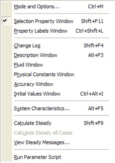
The model menu depends on the mode in which you are operating. Below the Model menu in engineering mode:
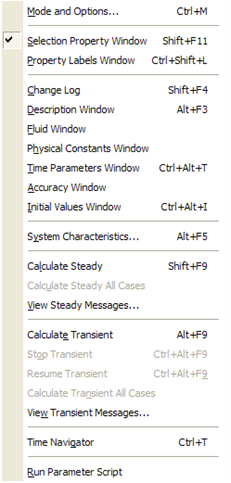
In Transient mode the model menu appears as follows:
See also
2.14.2. Mode and options
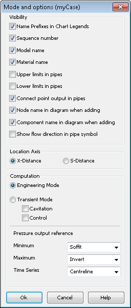
This dialog allows you to select for this case the visibility of some properties and the calculation mode of Wanda.
Default all boxes of the visibility properties in the upper part of this window are checked and thus visible in the Property Window (or chart). By un-checking the boxes you can make the properties invisible.
The “Upper limit pressure” and “Lower limit pressure” fields are only applicable for the PIPE’s. if these fields are checked, the PIPE input properties are extended with extra input fields and become visible in the pressure and head location charts.
With the field “connect point output in pipes” checked, the pipe output is extended with the quantities in the begin and end H-node. The advantage is that the time series in these points are available directly without specifying a value in the “location” field.
Adding a new H-component or H-node automatically the name of the new object is displayed in the diagram (the display box in the property window is “checked”). This display function during adding can be controlled by the two “.. when adding” boxes.
The checkbox “Show flow direction in pipe symbol” can be used to show arrows on top of pipes (see figure) in the flow direction. This can be helpful to determine how the flow is distributed in complex networks. For water hammer pipe the flow direction is the average of the velocity at the connect points. To enable or disable this, the simulation has to be rerun. When the absolute velocity is lower than the convergence criteria, no arrow is shown.

The lower part of this window contains mode and options related to the computations. The radio button allows you to switch between Engineering mode and Transient mode. In Transient mode you can activate three options by checking the boxes.
If “Cavitation” is checked, cavitation is taken into account during the transient calculation. See Theoretical and mathematical background. If “Control” is checked (must be part of your license), the control scheme is part of the transient calculation. If not checked only the hydraulic components are calculated.
The “Pressure output reference” had to do with elevation reference is used for the pressure computation. For more information about this subject see the PIPE component: PIPE.
2.14.3. Property labels
The WANDA user-interface is in (UK)-English. For all output the English terms are used, such as “cavitation volume” and “discharge”. This can be a problem when reporting to non-English clients, or preferring other (US)-English words. To solve this ‘language problem’, the user can define another description for any component property. The user definitions become part of the case and can be also saved in template files to build your own “property library”. All output tables and figures can be represented with property labels that best correspond to the hydraulic vocabulary of the user or user-clients. To change back to the default value, delete the user specified one.
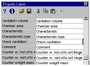
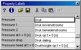
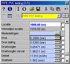
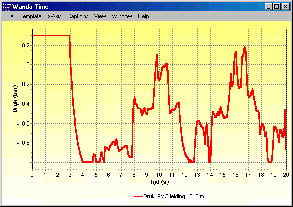
The property labels window show all property labels which are available. It is recommended to translate it once and store this translation in a property template file.
The next time you open a new case, you only have to read these labels from file.
The translated labels are stored in the case. If you have more than one case open, the latetst case defines the current label setting, because the userinterface can handle only one translation.
2.14.4. Change Log (Shift+F4)
For every case, a log-file is created in a rtf-file. This log-file can be modified via the Model menu. The log-file also keeps track of the ‘save-as’-actions, such that the complete history of the case can be seen. Upon closing the case, the user can make some extra comments in this log-file.
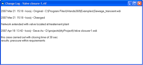
2.14.5. Hydraulic input of your model
The hydraulic model consists of the diagram with its H-component and H-nodes. Properties of these objects are specified using the property window.
To run steady and transient, the model requires some general data. This data is divided in 5 parts:
Description: enter a description of the current case
Fluid: specify various physical properties of the fluid
Physical constants
Time Parameters: enter the time-step, simulations time, etc, necessary for the computation of steady- and transient-state flow
Accuracy
2.14.5.1. Description…
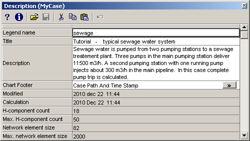
The case name can contain certain information about a case simulation. However, the length of the case name is too short to allow a general description. The description window in the model menu can be used to describe the simulation in more detail. The user may give an elaborate description of the system simulated, such as the piping network, the flow process, the objective of the simulation, and the main results.
The “legend name” field is used in the chart legend (max 8 char. long). The “Title” field (60 char. long) is used as header in charts and input and output reports. The “Description” field (1000 char. long) is for additional comment. You create a new line by pressing alt+enter (like Excel).
The “Chart Footer” field is used for printing an identification string in time and location charts. There are several options for the content of this footer text varying from a full path and case name including simulation date/time to only the case name. With option “None” the footer text is empty.
2.14.5.2. Fluid…
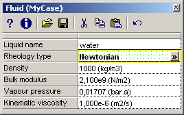
In the fluid window the physical properties of the fluid are specified. The contents of this property window depend on the mode you are working (Engineering/ Transient) and the domains you are authorized for (Liquid, Heat). For instance, the “bulk modulus” is applicable in transient mode only.
By default the values valid for water at ambient temperature are given in the table. The fluid name is purely documentary and has no effects on the computation. In case other fluids or water at a different pressure/temperature rating are simulated, the values in the table have to be adapted accordingly.
Choosing Rheology type = Slurry (Optional licence feature) shows the required input parameters for the Herschel-Bulkley model.
In the Heat domain the fluid properties are temperature dependant. Therefore a table has to be specified. A default table can be retrieved from the property templates subdirectory (part of the Wanda program directory)
2.14.5.3. Physical constants…
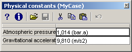
In the window above you can specify atmospheric pressure and gravitational acceleration for your hydraulic model.
2.14.5.4. Time parameters…
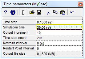
The time parameter window is applicable in transient mode only.
Time parameters must be entered for each transient calculation.
The choice of the time-step demands careful consideration. A large time-step generally saves computation time, but the accuracy in the computed results could be low. Choosing a small time-step has the opposite effect. The choice should be based on the dynamic process simulated and the properties of the pipes and the fluid in the system.
The size of the output file depends on the size of the network (number of elements) and the number of time steps. The estimated size in mentioned in this window. Note that the maximum file size is 2 GB. You will get a warning if this size will be exceeded.
You can reduce the size of the output file by setting the Output increment to a higher value. Setting the Output increment to 10, for example, reduces your output file with a factor 10. If you play Movies or view time series only every 10th time step is displayed. The extreme values charts do remain correct (i.e. based on all simulated time steps).
It is possible to show the results during the simulation. The “Refresh Output Interval” is the refresh rate in real seconds; all open charts en property output windows are updated automatically with this interval. Looking to the progressing results, you can interrupt the simulation when you find them unsatisfactory.
The Restart point interval controls how often a restart point is created during the unsteady simulation. The Wanda simulation can be restarted from these points in the simulation. This greatly reduces simulation times when the user changes an action table in a large model. The restart point interval must be larger than the output increment and must be a multiple of the output increment.
2.14.5.5. Accuracy…
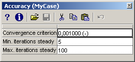
These parameters are used for determining the end of the iteration process to solve the non-linear hydraulic equations in the steady state and at the boundary conditions in the unsteady state. If the relative difference for each element between the last solution vector and the previous iteration is smaller than the convergence criterion, the solution is assumed to be converged.
For steady state calculation it can be necessary to prescribed the minimum number of iterations to get a satisfied and fully converged solution.
To prevent the program for looping if no convergence can be obtained, a maximum number of iterations is introduced.
Normally the default values has not to be adapted.
2.14.6. Initial values
The PIPE component (Liquid module) use a table with local losses.
You can define your own default values for the local losses. These values will be used as default settings for each pipe.
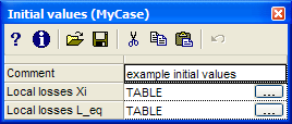
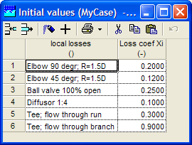
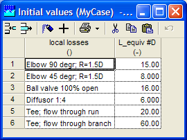
Wanda is delivered with settings as given above. These settings are saved in a template file “default.ptf” in subdirectory “Initial values”. If these settings do not satisfy your company settings, change the contents and save it (using the save button) to the default.ptf-file.
Each time a new case is opened, the contents of the default.ptf file if copied to the internal data structure of the case. Changing these case settings does not affect the global settings in the template file.
Each time a Pipe with local losses is added to the diagram, the current case settings are copied to the property data structure of the Pipe. Editing the Pipe properties does not affect the case settings.
2.14.7. System characteristic chart
This option creates a chart containing several assembled pump characteristics and several system characteristics
This is done in three steps:
create an assembled pump characteristic
create a system characteristic
combine pump and system characteristics in one chart
These steps are carried out using the window as depicted below.
By default the directory name of the current case is shown. It is possible to choose another directory using the browse button.
If you have never defined a chart before, you first have to specify a new one. Press the New button and specify a chart title. The dropdown box shows all available chart titles created before.
The two large list boxes show existing characteristics. If they are empty it means that no curves have been generated yet.
All characteristics are stored in ASCII files with fixed extension (.wpc for pump characteristics and .wsc for system characteristics) These files are stored in a subdirectory of the current case directory. This subdirectory name is specified by the user and this name is used as title for the chart to be assembled.
2.14.7.1. Assembled pump characteristic
To create an assembled pump characteristic you first have to select one or more pumps in the diagram. The caption of this window shows the number of selected pumps. Then press the Create button in the assembled pump characteristic box and the program will generate the assembled curve. To identify this curve you have to specify a unique label. The program suggests a label based on the model name of selected pumps, which may be changed by the user. In the chart this label will be used as legend text. The label is also used as file name (filename.wpc in subdirectory casechart label)
To delete an existing curve, just select the curve label in the box and press the remove button.
2.14.7.2. System characteristic
The system characteristic describes the head as a function of discharge at a certain location. To determine this function the H-component QSCHAR must be defined in the diagram. The QSCHAR represents a set of pumps.
Pressing the Create button in the system characteristic box activates the calculation. In fact this is a repeating calculation of Steady with different discharge steps. Steady takes 25 equidistant steps beginning with 0 m3/s until Qmax m3/s. Qmax is an input property of QSCHAR. To activate this calculation all input of the hydraulic network must be complete and satisfy the validation rules. If the “Create” button is disabled, check the input using the selection menu item “select first (all) invalid components”.
In contrast to the normal Steady calculation, it is not necessary to specify the status of checkvalves (or other solution dependent properties of other H-components) in the right way. During calculating the Q-range the checkvalve can change from “procedure phase”. This change is automatically carried out.
See H-component QSCHAR for more information.
To identify this curve you have to specify a unique label. In the chart this label will be used as legend text, so use a meaningful name. The label is also used as file name (filename.wsc in subdirectory casechart label).
To delete an existing curve just select the curve in the box and press the remove button.
2.14.7.3. Create combined chart
To create a chart with pump characteristics and system characteristics select the applicable characteristics in the list boxes.
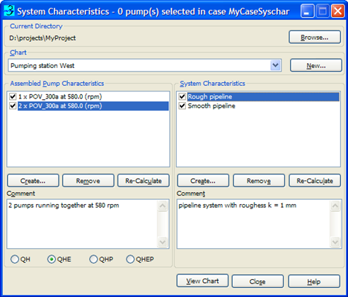
Then press the “View chart” button.
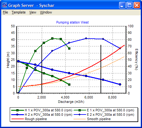
The chart appears in a separate window. To create another chart, first deselect the items by clicking on them a second time and select a new set. Press the “View chart” button again and a new window appears.
2.14.8. Calculating your model
2.14.8.1. Calculate steady
When a hydraulic model is completed and the hydraulic specifications are given, the user tends to go immediately for a run of the steady-state and transient flow computations. However, input errors are often inevitable. Causes for the errors can be associated with the complexity of the system modelled, incidental errors made by the user or lack of experience with WANDA. Therefore, it is useful to check the correctness of the hydraulic model and the input hydraulic data before make any computation.
See also:
Calculate steady in WANDA is used to compute the steady-state flow in the pipeline system. When you choose this option WANDA starts to calculate the steady state in a separate console program:
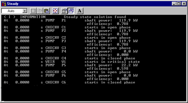
The progress of the steady-state computation is displayed The computation is successful when the message is Steady-state solution found is displayed:
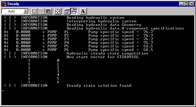
After computation these messages can be viewed using View steady messages… from the Model menu.
Steady-state flow equations are non‑linear equations, and are solved iteratively. A set of initial values of the flow variables (a start vector) is used for the iteration. When no convergence is found using one vector, the computation continues with a new start vector. A total number of 9 start vectors are designed in the module. In case they are exhausted and no convergence is found yet, WANDA terminates the computation and issues an error message. Details about the mathematical model and numerical methods used to solve non-linear equations can be found in the section Theory behind WANDA 4 (General form of the equations).
Messages generated by the module can be classified into five categories. The computation is aborted in case of a terminating error message. Certain categories of messages can be suppressed in the display window using the message threshold in the general computation data.
2.14.8.2. Calculate steady all cases
It is possible to open several different cases. By choosing this option all open cases will be calculated.
2.14.8.3. View steady messages…
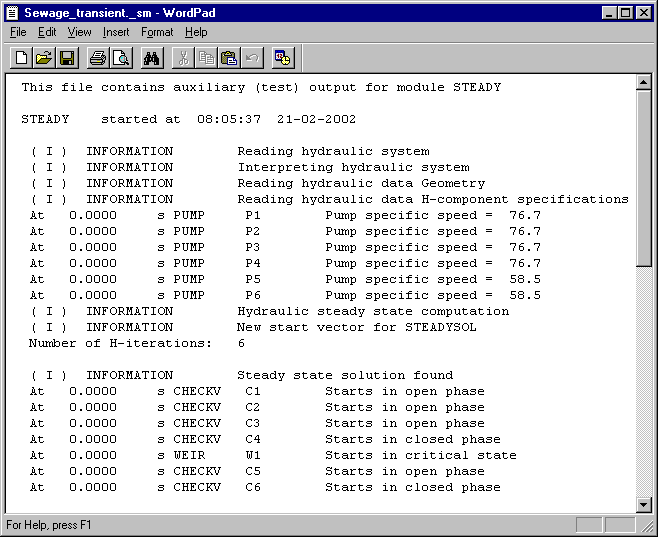
Above you see an example of the messages after a steady computation of your model. WANDA 4 shows these messages in the Notepad. In this way it is very simple to save the messages as a text document and use them for reporting purposes.
2.14.8.4. Calculate transient
Calculate transient in WANDA is used to compute the unsteady state in the pipeline system.
The progress in the transient state computation is shown. Program messages are also displayed.
Messages generated by the module can be classified into five categories. The computation is aborted in case of a terminating error message. Certain categories of messages can be suppressed in the display window using the message threshold in the general computation data.
Calculate transient generates two files. One of the files has the extension “__R”, and is an interface file between the module STEADY and TRANSIENT The other file, with extension “_UM”, is the message file where all messages generated by module TRANSIENT and the component procedures are stored.
The computation can be stopped at any time and resumed later (see Resume transient).
2.14.8.5. Stop transient
This option interrupts the transient calculation. Results of the simulation so far can be analysed. The user may resume an interrupted transient calculation using the menu option Resume transient.
2.14.8.6. Resume transient
This option continues the transient calculation.
2.14.8.7. Restart transient from
Allows the user to choose a restart point and restart the transient simulation from that point.
2.14.8.8. Calculate transient all cases
It is possible to open several different cases in WANDA 4. By choosing this option, all open case will be calculated. This option is useful if you want to calculate several large models (e.g. by night). Verify that you have sufficient disk space available. You can adjust the size of the output file without losing calculation accuracy by setting a time output increment in the Time parameters window.
2.14.8.9. View transient messages…
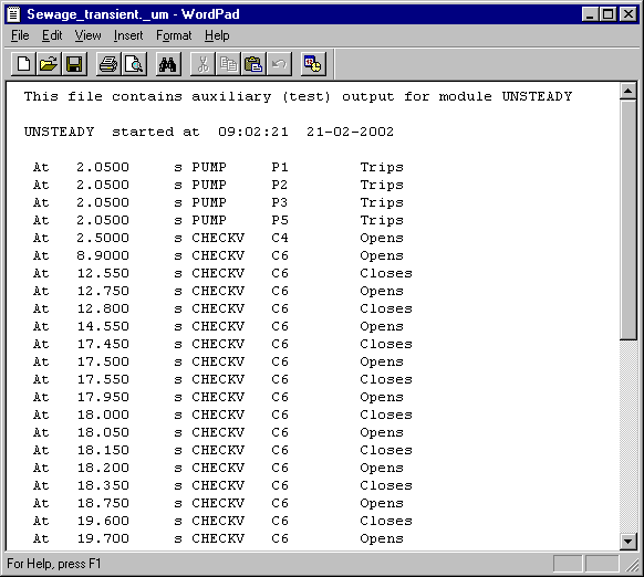
Above you see an example of the messages after a transient computation of your model. WANDA 4 shows these messages in Notepad. In this way it is very simple to save the messages as a text document and use them for reporting purposes.
2.14.9. Run Parameter Script
2.14.9.1. Concept
In many projects, different scenarios (e.g. flow rate, operating pressure etc.) and settings (water level in surge vessel, valve closure speeds etc.) need to be simulated. Often it is useful to start from the same original (mother) case. The Parameter Script in Wanda is the tool to use for this kind of projects.
The concept of the Parameter Script is that there is one (original) mother case, from which several child cases are created and run. For every child case the user defines the input which needs to be modified. To enable quick review of the results, extreme output values for every child case can be saved in a CSV-file. For further details, the user can open the child cases of interest. Since the Wanda 4.2 release, an Excel tool is included to simplify the use of the Parameter Script. In this Excel file, all input values and required output results are listed. The advantage of using this Excel file is that:
It is easy to distinguish between different cases and manage a sensitivity analysis.
It is easy to open the different child cases, since for every child case a shortcut is added.
All internal Excel functions can be used to create the values for the input parameters.
Although the use of Excel is very convenient, the Parameter Script can also be used with any text editor.
2.14.9.2. Main steps
In the Wanda example folder (“File -> Open Example -> Parameterscript”) an example of the Parameter Script can be found (“Sewage_transient_WPS.wdi”).
To use Parameter Script the following steps need to be taken:
Create a mother case using the Wanda user interface.
Create a Parameter Script file: “MyCase.wps”. This can be done with help of the parameter Excel file, which can be found in Wanda4/tools folder, or by manually creating a “Mycase.wps” file by using a text editor like Notepad. Note: the name of the Parameter Script must be equal to that of the mother case file.
Start the Parameter Script via the pull-down menu in Wanda (Model menu -> ‘Run Parameter Script’).
Review the results in the CSV-file. Child case can be opened in the Wanda user interface, when the option for saving the child cases is selected.
2.14.9.3. WPS file creation
The WPS file can be created via an Excel file. The Excel file consists of three sheets: Cases, Output and Readme. The latter contains the same information as given here and is added as quick reference. Below an explanation of the other two sheets is given.
Cases sheet
The Cases sheet contains all input information, like the parameters to change and the value of these parameters.
The top three rows are the header rows. From row four downward, information for every child case is given.
First column “Case number” and second column “Case description”: These rows can be used to support organize the Parameter Script. Any text string or number can be used but it can also be left empty.
Third column “Include”: It is used to select the case which should be (1) included in the Parameter Script run and which not (0).
In column four “Name”, the mother case can be saved and the extension for every child case is given (the child case name becomes: mothercase_childcase).
In the columns after the Name column, the input parameters are given. In the top row the Name of the component (example “CHECKV C5”) or a Keyword is given. In the second row the Property to change (“Initial state”) is given. This is the English Property and case sensitive.
The set-up of the parameter Script excel file gives the user a lot of freedom for extensions (and deletions). Almost all columns may be deleted, moved and copied. However, the two columns “Include” and “Name” may not be deleted.
Please note the following:
All input value should be given in the unit system of the mother case.
It is also possible to use Excel functions to calculated values or to get them from different sheets (e.g. VLOOKUP function) if required.
Components can only be disused and not used. Meaning: all components which are listed in the in- or output should be used in the mother case.
Be careful in using disuse, since this can cause the Wanda model to be invalid and resulting into a crash of the calculations.
The length of a pipeline should not be changed, since this will result in unexpected output and possibly a crash of Igrafix.
Using the keyword: GENERAL, the fluid and physical properties can be assessed, just as the simulation time parameters, and the simulation accuracy (see also: Model menu – Fluid Window / Physical Constants Window / Time parameters Window / Accuracy Window).
Drop down list ( e.g. “Initial state”) can also be changed. The number of the item in list requested should be given as input value (e.g. “4” should be used if the valve should be set to initial discharge).
Tables (local ksi losses, pipe profile, action table, QHE-characteristics) cannot be adjusted with the ‘Parameter Script’.
To run Parameter Script again, check whether the result-file (csv) is closed.
Output sheet
The Output sheet contains three columns. The first column gives the name of the component or Keyword (e.g. “PG1”) for which an output should be saved. The second column contains the Property for which the output should be saved. The third row states whether the minimum (“MIN”) or maximum (“MAX”) should be saved. Next to this the following SAVE keywords can be given:
SAVECASE: for each child case the .wdi-, .wdo-, .wdx–file is saved. These child-cases can be opened with Wanda.
SAVEMSG: for each child case the ._sm-file (see: Model menu – View Steady Messages), and the ._um file (see: Model menu – View Transient Messages) is saved.
SAVEALL: combination of SAVECASE, SAVEMSG.
REBUILD_CSV: The CSV file is rebuilt from the existing child cases. This is useful when other output is required after the simulations have been performed.
Creation of the WPS file
After the Excel sheet is filled, click on the button “Create wps” in the Cases sheet. Please note that macros need to be enabled. Follow the instructions. At the end a WPS file is created. This files consists of 3 blocks:
Input parameter definition: defining the parameters that the user wants to change; via the Keywords of the objects and the Property description.
Output results definition: defining the results of each individual child case that the user wants to have saved; via the keywords of the objects and the property description. Using the SAVE-keywords the child cases themselves can be stored.
Run definition: lists for each child case: The name of the child case and the input values of the input parameters as defined in the Input parameter definition.
Every group starts with the number of in-, outputs or cases which are given. The example below shows this syntax.
The final step is starting the parameter script from the Wanda User interface (Model -> Run Parameter Script) After the Parameter Script runs are finished, the csv-file with the results is opened automatically. Depending on the chosen option for saving of simulations, the child cases can be inspected (or not).
2.15. Reports Menu
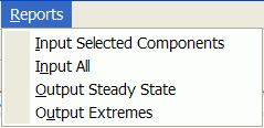
The Reports Menu allows you to save and edit all input and output of your hydraulic model, for the purpose of reporting.
After the hydraulic model has been created and the input data have been entered, the user may need to have a full report of the input data. The report can be used either for inspection of the numerical values of the input data, or for documentary purposes.
Likewise the user wants a summarized report of the output after a successful calculation
WANDA generates the reports in a compact spreadsheet format (tab separated ASCII file). After generating WANDA starts automatically the default spreadsheet program associated with “csv” extension. The spreadsheet output can be further arranged outside the Wanda program.
The components are ordered by name. Each row contains all input or output parameters. Because a cell can contain only scalars, the tables with input items are displayed separately. A unique table identification is used for reference.
2.15.1. Input selected components
The input report contains only the input specifications of the components selected by the user. This means, that if you want a report on a special group of components you have to select them by using the selection builder (ALT+F7) or the selection menu.
All other input data such as fluid properties, network connectivity is ignored.
2.15.2. Input all
A full input report contains the following information:
case descriptions
general computational data
fluid data
hydraulic properties of all components, including tables
network connectivity
This option provides an overview of the input of all data in the model. This report can be used for backup purposes (printed hardcopy of your model input).
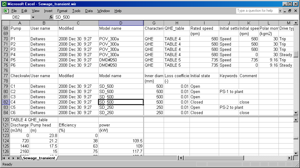
2.15.3. Output steady state
This output report shows all calculated properties of all components of the steady state computation.
Because the components are ordered by type, you get a compact table of standard output (depends on the physical domain) and component specific output.
Because the component messages are text tables, they are displayed separately. If you want a chronological list with messages, access the Steady messages report (model menu).
2.15.4. Output extremes
This output extremes report shows all minimum and maximum calculated properties of all components after the simulation has been executed. Also the point of time when the extreme value occurs, is included
Because the components are ordered by type, you get a compact table of standard output (depends on the physical domain) and component specific output.
Because the component messages are text tables, they are displayed separately. If you want a chronological list with messages, access the Transient messages report (model menu).
2.16. Pump Energy
2.16.1. Overview Pump Energy module
The Pump Energy Module is part of WANDA Engineering. With this module you can calculate the most efficient use of pumps in a pumping station based on a specified delivery pattern and the system characteristic. The program gives you the total energy consumption in a specified period regarding the specified pump operation.
The Pump Energy module is not a separate window but is a combination of a few components. These components are explained in detail in the Help on Overview of Liquid components.
Hydraulics components that must/can be used in Pump Energy are:
PUMP |
the pump model |
PUMPSCEN |
Pump scenario to specify the operation of pumps |
SYSCHAR |
System characteristic |
Q_FREQ |
Discharge Frequency |
Q-PATTRN |
Discharge Pattern |
One or more of these components are placed in the diagram. The module needs only one SYSCHAR and one or more PUMPSCENs and PUMPs. The use of Q_FREQ and Q_PATTRN is optional. These components define the time; without one of these components no energy consumption can be calculated. The system characteristic is a Q-H table defined by the user; it may be retrieved using the System Characteristic module. In that case the curve data must be copied (using the clipboard) from the system characteristic chart to the SYSCHAR input table.
2.16.2. Schematic aspects
The figure below shows an example of a diagram to perform a Pump Energy computation.
The group of pumps represents the pumping station; other components like valves, checkvalves and pipes may occur in the system but doesn’t have any influence.
Only one (not-disused) SYSCHAR must be present; More than one PUMPSCEN is allowed, so you can compare different scenarios at once. The connections between the different components are not necessary; the PUMPSCEN component carries out the computation based on the specified data of the active PUMP’s, SYSCHAR and (optionally) Q_FREQ/QPATTRN. The computation will be done directly after an input is done; that means that changing a parameter, the new results are directly available.
Inconsistency in the diagram or input is communicated by the message property of PUMPSCEN.
The PumpEnergy components PUMPSCEN, Q_PATTRN, Q_FREQ and SYSCHAR are ignored by the WANDA processes “Steady” and“Unsteady”
The dialog between user and program is done by the diagram: the pumps that must be evaluated are located in the scheme. Only the input fields QHE table and rated speed are necessary, the other values may remain empty.
In the PUMPSCEN component a scenario of operation is defined. The scenario table contains all (not disused) pumps.
The user has to specify in which discharge range a pump or group of pumps are in operation. The pumps are speed controlled (a “0” is specified) or runs at a fixed speed (the concerning speed is specified). In above example the first 3 stages are operated with variable speed pumps, 1 different pump for each different case. The next stages are operated with one or two pumps at fixed speed and one at variable speed.
The PumpEnergy module calculates for the whole range of discharges the efficiency and power of each pump. In case of variable speed pumps, the necessary speed is calculated to satisfy the duty point according the system characteristic. All important pump properties, like discharge, head, speed, efficiency and power, can be visualised.
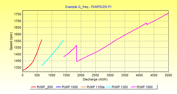
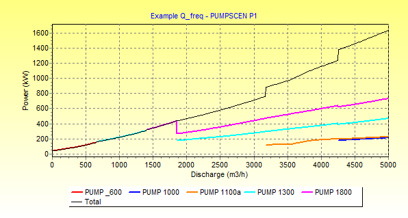
If we know how many hours the pumps operate, the energy consumption can be determined.
The time aspect can be specified in two different ways:
a histogram annotation that tell us how many hours a certain discharge is delivered in a certain period (Q_FREQ)
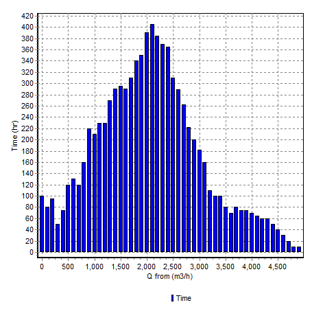
a discharge pattern as function of time (Q_ PATTRN)
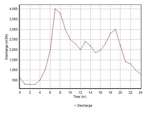
The energy consumption is displayed in the scenario table and can be visualised in a chart
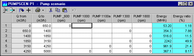
More information about the individual Pump Energy components is explained in the Help on Overview of Liquid components.
2.17. Tips for WANDA 4 users
2.17.1. General tips
Read the manual.
Always make a (temporary) local copy of a Wanda case stored on a network server or removable drive. Data is loaded dynamically so the access time determines the speed of Wanda. The access time of a local drive is about 100 times faster.
Use the context sensitive menu (right mouse click) in the diagram and property window to get fast access to frequently used options.
You can open a Wanda file from a file manager by double clicking the wdi-file or dragging a wdx-file into the Wanda diagram window.
You also can drag a file to the windows taskbar. Keep the mouse button down until Wanda becomes visible and move the dragged file in the diagram window.
You can use your favourite text editor (Messages, Reports) by associating the txt-extension to your favourite text editor. (‘View.Options.File types’ menu item in the windows file explorer).
Use the same model name for components that share the same specifications (properties).
Use keywords to group a set of Components.
The information in every window reflects the current situation. You don’t have to re-open windows to update them.
If you are not interested in the output at every single time step check the ‘Show Extremes’ option in the Model menu.
Press F11 to switch the focus between the property window and the diagram window.
Wanda works best at a resolution of 1280x1024 and a 19” monitor or better.
Sometimes the diagram doesn’t become visible when you click the taskbar. Right click the Wanda button at the taskbar and choose restore.
You can resume transient with a different output increment.
Make property templates with fluids that you use frequently.
You can delete the wdo-files of cases to create more disk space. When you delete the wdo file of a case only the output is deleted. If you send a case by mail create a zip file with the wdi and wdx file. These three files are the only files needed.
Learning the keyboard and mouse shortcuts will save time when you are using Wanda frequently.
If you have additional tips lets us know.
2.17.2. Shape libraries
You can customise the Wanda Hydraulic and Wanda Control shape library.
You can add extra custom shape libraries.
DON’T DRAG WANDA COMPONENTS FROM THE DIAGRAM TO THE SHAPE LIBRARY.
You can copy shapes from one shape library to another. Use the right mouse button to cut/paste.
Copy shapes between shape libraries one by one. If you don’t, Wanda will crash due a bug in iGrafx.
It’s easier to collapse the gallery than closing the gallery. Use the button ‘>’ left from the ‘X’
You can resize the buttons in the gallery (shape libraries) by moving the right-down corner of a single button.
2.17.3. Diagram general
The mouse cursor indicates what happens when you click (Selecting, Moving, Dragging a line, Inserting a new component).
Hold the SHIFT-key down while clicking an object to extend a selection by a single object.
Hold the SHIFT-key down while clicking a selected object to shrink the selection by a single object.
You can drag a selection rectangle to select multiple objects at once.
You can extend a selection by multiple objects at once by dragging a rectangle while the SHIFT-key is down.
If you change the line style / weight / colour while no objects are selected the style is applied for new lines and shapes.
You can visualise a property in the diagram by clicking its checkbox in the property window.
If you toggle the menu item ‘show extremes’ the output properties in the diagram are also changed (delay 3 seconds).
If you move the slider in the time navigator the output properties in the diagram are also changed (delay 3 seconds).
Use a postscript printer driver when the diagram or chart is not printed correctly. (HP delivers also a postscript driver for all it’s laser printers).
Right click at a component or connection to popup extra property windows.
Deselect all objects before printing to prevent red circles behind objects.
Before you copy the diagram selection to another application (e.g. MS Word) first press the ‘A’ button in the property window. This prevents that a red circle behind a component is also copied.
Some Nvidia video drivers don’t work properly when using iGrafx professional. Wanda crashes during starting or directly after adding a component. Download the newest video driver from the Internet. It’s still possible that background pictures hide the diagram partly. Use a separate layer for the pictures and hide this layer during editing.
By pressing CTRL+F6 you can quickly switch between open diagrams.
To navigate in large scheme’s, use the split window mode. The upper part is used for navigation, the lower part is used for editing.
2.17.4. Diagram editing
If you are dragging a selection you can cancel this operation by pressing the escape button before releasing the mouse button.
Hold the CTRL-key down if you want to copy a selection instead of moving a selection.
You can draw components like vectors (Wanda 2 functionality). Select from the shape library the component type you want to draw. Press the shift key and keep it down. Right click the diagram background to switch to the line draw mode. Draw a line. The selected component in the shape library is now automatically inserted in the middle of the new line. The H-nodes (connection lines) at both sides (only upstream side in case of a supplier type) are automatically generated. When you are finished with vector drawings you can release the shift button.
You can hide/unhide the grid dots with the sub menu “Grid” in the “Arrange” menu.
Editing is easier when you first ‘snap to grid’ all components. If you convert a Wanda 2 case the diagram size is reduced with 25 percent. Due to this reducing the objects are not ‘snapped to grid’.
If you want to connect a connection line in the middle of another connection line which is very short (less than 1 cm), the green blinking connect point snaps automatically to the end points. Accept this location while the WANDA program moves it to the centre of the line.
If you want to move a text (e.g. name) of a component/node first select the tab “Text” in the diagram window.
Don’t move a selection to another document.
Copy the selection first and delete the original selection afterwards.
You can align components by using the blue rectangle. When you move a component across another component this component is marked with a blue rectangle. Keep the mouse button down and move the component to the wanted location. When you release the mouse button the component is snapped to the position that’s exactly aligned with the blue marked component.
You can shift + right-mouse-click at the diagram background instead of pressing the line tool button. Press twice to toggle between direct line and right angle line
You can ctrl + right-mouse-click at the diagram background instead of pressing the last selected shape at the shape library.
By adding extra vertexes to a connection line you can route the line to another path. You can add extra vertexes to connection lines by pressing the right-mouse button while you hold the SHIFT-key down.
If the diagram isn’t displayed correctly or the selection isn’t the same as in the property window press F5 (Refresh) while the diagram is active.
2.17.5. Diagram layers
Use a separate layer for pictures (backgrounds). You can quickly hide this layer to increase the scroll/zoom speed and reduce flickering (layer manager, activated by right click at layer tab). The background must be the first in the list (use move up button), otherwise the components are not visible.
Move (a group of) disused components to a different layer. You can toggle the printable option when you right-click the tab. When the option is unchecked the layer is not visible when you print the diagram.
If you want to edit multiple layers choose edit all layers and lock the layers you don’t want to edit.
Right click at a layer tab to see a context menu. With this menu it is easy, among other things, to hide and unhide layers. It’s important that the layer-tab that you want to hide is not active.
2.17.6. Diagram routes
A route is an unambiguous and continues sequence of H-components; this route can be specified with a keyword.
You don’t have to select all the component in your route one by one. Select the first component in your route. Now select the last component in your route while holding the Ctrl and Shift key down. The other components and connections in the route are now automatically added to the selection. It’s important that the components are connected before you select the route.
If the route Wanda chooses isn’t the way you had in mind you can select extra components before you select the last component by Ctrl+Shift+Click. Now Wanda is forced to choose a certain path. Keep the Shift key down while you select the extra components.
Use the ‘align route’ menu option or (CTRL+ALT+A) to align a route in a fast way to another direction. First move component A to the wanted position, then move component Z to the wanted position. Choose ‘align route’ to redirect all components between A and Z in a straight way.
2.17.7. Property windows
If you select multiple components/nodes you can inspect multiple properties by pressing the ”range” or “spreadsheet” button in the property window.
To select/deselect properties in a property window, press the space bar, click at the description or drag the mouse in the input field.
You can drag/drop selected properties from one property window to another property window.
Every component/node also has hidden properties. With the hidden properties you can see the connectivity used by steady and transient. To unhide the invisible properties press the pause key while a property window is active (may be useful in case of ‘strange’ problems).
If you are editing a text property you can insert a line break by pressing ALT+ENTER (same way as in Excel).
You can quickly move to a property in the property window by pressing CTRL+ALT+”First character property name”.
If you want to edit a part of a property value first press F2 or enter to become in edit mode.
You can open a table or chart window by pressing enter at the particular property.
Use the menu items ‘Add keyword to selection’ and ‘Remove keyword from selection’ to update the keyword list when you have a multiple selection.
Export your frequently used properties of components to property templates. Now you can easily reuse components between cases (or colleagues).
You can load a property template file from the file manager by dragging the file into the info/unit section of a property window (I-button must be pressed).
You can see the Wanda help while editing the properties by setting the online help ‘always on top’.
2.17.8. Tables and tabular views
To show a tabular view, select one or more properties (marked as blue) in the property window and press the ”spreadsheet” button.
You can print a table or tabular view by a right double click at the grid. An Excel like window appears. Choose ‘Page setup.’ in the file menu to fit the print to n by m pages (landscape or portrait).
While you are defining the pipe profiles of the pipes in a route you can open the Head chart to see the profile of the complete route. This chart is updated while you are changing a pipe profile in the route.
The contents of the spreadsheet can be copied to Excel using the clipboard.
If copying data between Wanda and Excel fails, check the regional settings. The decimal symbol must be set to “.” (dot).
You can open multiple spreadsheets at the same or at different cases.
To change rows and columns, press the rotate button.
When you press CTRL+F4 the window closes and the focus returns to the property window.
2.17.9. Charts
Use the most recent printer driver when charts are not printed correctly.
You can drag/drop chart-series buttons (also from different cases) to a single chart window (also when a movie is playing).
Use an applicable short name if you have a multiple case chart. The short name is added between brackets to the series title. You can change the short name of a case in the description window.
Make you own chart templates if you are not satisfied with the default graph settings.
There are four groups of templates: Time series templates, Location templates, table templates and system characteristic templates. Templates can be shared or copied to another group by copying a local template to a global template.
Before saving a chart template first check the ‘captions.absolute’ menu item. You see now the quotes that are not converted to keywords. These quotes are saved absolute to the template. You can choose ‘Reset to default’ to remove all absolute quotes.
You can see multiple location series at once (Route) when clicking a chart button. First make a multiple selection of pipes. All the pipes in a selection must have the same flow direction. Also select components between selected pipes.
You can see multiple time chart series lines at once when you click a chart button. First make a multiple selection of components with the time series you want to see.
Fill the location property if you want to see pipe time chart series instead of pipe location chart series.
- Use the right mouse click to open a “selection chart window”. This is a global window wherein each selected property chart is drawn.The advantage is that now only one chart window is used for all time series and one for all location series.
You can drag a chart button to a chart that already has that location property. This location series is frozen at the active time step. Also frozen series are automatically updated when you run steady/transient again.
You can quickly zoom into a chart by dragging a rectangle from left to right.
You can quickly undo zoom by dragging from right to left.
You can scroll the chart down/up and left/right by moving the mouse while the right mouse button is pressed.
Line patterns don’t work fine if the series points are close together.
2.17.11. Selection builder
If you don’t specify a value and using the ‘=’ operator Wanda searches for empty/missing values.
If you specify a ‘*’ as value and using the ‘like’ or ‘=’ operator Wanda searches for every value.
You can use the hidden colour property to select all objects with the same colour.
2.18. Frequently asked questions
2.18.1. Manage files
Questions |
Answers |
Which files are necessary for backup purposes |
All input of the case is stored in the wdi and wdx file; all other files can be generated again performing the calculation. |
I can not save my WANDA case |
You are probably viewing a WANDA case with components that are not part of your license. You can only save cases that can be built with your license. Press F10 to select the unlicensed components. |
2.18.2. Gallery/Shape library
Questions |
Answers |
The gallery is not visible |
Go to menu “view” and mark “Gallery” as visible, or activate the right mouse click menu and check “shape gallery” |
One of the shape libraries is not available in the gallery Hydraulic (no tab visible) |
At the gallery tabs, click the right mouse button; choose “open palette” and select form the group “Wanda components” the required subject |
The component tooltip text is partially not visible, it disappears behind the property window |
The property window is always “on top”. Move the gallery window to the left side of the diagram. |
2.18.3. Route
Questions |
Answers |
How can I create routes? |
There are several ways to select a route (a route is a concatenation of 2 or more H-components). A very fast way is click first H-component followed by CTRL-click of last required H-component. WANDA selects the shortest route. If a particular H-component must be part of the route, add them to the selection before creating the route. |
See also: Select route between selected components or use the short cut menu.
2.18.4. Diagram / Layers
Questions |
Answers |
It is not possible to move the text labels in the diagram. |
The model is built in different layers. Choose the “text” layer tab at the bottom of your WANDA window to change the position/font/size of the text. |
How can I put a map as wallpaper to my diagram? |
On the Arrange menu, point to Layers, and click Add Layer. The new layer is added in front of the current layer and becomes the new current layer. The wallpaper layer must be moved up to the top On the Insert menu, point to Picture and specify a bitmap picture from file Resize the picture to the desired size |
How can I rotate or flip a component |
Press the right mouse button in the diagram and choose “Arrange”, or use the “Arrange” option from the menu bar. Flip and rotate buttons can be made visible via “view/toolbars” menu, check the draw toolbar. |
I want to draw a H-component in another direction than from left to right. Is that possible without using the flip/rotate? |
In vector line mode you can draw a H-component including its connection lines (H-nodes) in one movement. From the diagram short cut menu choose “Vector drawing”. Draw a line and the active H-component is placed in the centre of the line. Press Esc-key to leave the vector mode or choose from the short cut menu another mode. Another way to draw a component in a other (straight) connection is as follows: Draw the new component starting at an existing component by dragging the mouse. The new component is automatically arranged in the direction of the connection line drawn. |
Can I change the connection line type afterwards? |
Yes, a direct line can be changed to right angle line or just the other way round. A curved line can changed in a direct line or right angle line only |
2.18.5. Property window
Questions |
Answers |
What is the difference between the properties “Model name”, “Comment” and “Keyword”? |
In fact all of them are additional strings to describe the H-component. Model name and Keyword have particular intentions. Model name is introduced to define a particular identification of the H-component, e.g.: serial number, product ID, manufacturer name. In the next WANDA version this name will be used as default name for the property template file, when properties are exported or imported. Cases built with WANDA 1 and 2 uses the so-called common spec labels. These labels (used for data sharing) are replaced by a more generic data sharing concept; see also Properties of a Component. Common labels are assigned to the property “Model name”. The “Comment” field has no special meaning; use this for additional remarks. The “Keywords” field is used for quick selection. A H-component may have more than 1 keyword. Keywords are added and removed using the “Selection” menu; see Selection builder. Use keywords for Route definitions, groups of components (Pump station, High Pressure System etc); see Selection builder. |
2.18.6. Charts
Questions |
Answers |
How can I show more time series of the same quantity in 1 chart? |
Select first the wanted components (or H-nodes), then push the chart button of the wanted quantity. All series of the selected components are drawn in 1 time If you want to add new series, press the chart button and drag it into the existing chart. Release the mouse button and the new series will be added into the chart. |
Is it possible to show more series of different quantities in 1 chart? |
Yes, create a new chart by pressing the chart button. This property quantity is drawn at the left axis. Drag the chart button of the second quantity into the chart. This quantity is drawn at the right axis. It is not possible to have more than 2 different quantities in 1 chart. |
Is it possible to show more series of different calculations? |
Yes, create a new chart by pressing the chart button in case 1. Open case 2 and select the wanted component. Drag the chart button of the wanted property into the chart. To distinguish both series, use “legend name” from the menu “model/description window” |
How can I remove or change format from the footer text from the chart (in the footer text the case file and edit/run time is displayed) |
Choose from the model menu “Description window” Select form field “Chart footer” the required display text . |
How can I change the layout of the chart? |
Double click in the chart or choose menu “file/chart properties”. You become in the edit window at which all elements of the chart can be changed. The changed settings can be changed. See next question. |
How can I save the changed layout settings of a chart? |
To store these settings you must save it into a template. Choose from the Chart menu “Template”.followed by Save, Save As. or Save As Default. Using this Template menu you can switch between several layouts |
2.19. Important keys and shortcuts
2.19.1. Windows general
2.19.1.1. Keyboard
Ctrl + F4 |
Close document window |
Ctrl + F6 |
Next document window |
Alt + F4 |
Exit application |
Ctrl + Shift + N |
New |
Ctrl + O |
Open |
Ctrl + S |
Save |
F12 |
Save as |
Ctrl + P |
|
Ctrl + A |
Select all |
Ctrl + X |
Cut |
Ctrl + C |
Copy |
Ctrl + V |
Paste |
Ctrl + Z |
Undo |
Ctrl + Y |
Redo |
F2 |
Edit Text |
Shift + F10 |
Popup context menu (right click menu) You can also the special button between the right alt and ctrl keys |
2.19.1.2. Mouse
Ctrl + drag |
Copy |
Shift + drag rectangle |
Select and keep old selection |
Click |
Select |
Shift + click |
Select and keep old selection |
Right Click |
Popup Context Sensitive Menu |
2.19.2. IGrafx Diagram
2.19.2.1. Keyboard
Ctrl + Shift + 4 |
Align Top |
Ctrl + Shift + 6 |
Align Middle |
Ctrl + Shift + 8 |
Align Bottom |
Ctrl + Shift + 3 |
Align Left |
Ctrl + Shift + 5 |
Align Center |
Ctrl + Shift + 7 |
Align Right |
F5 |
Redraw diagram |
F2 |
Start (editing) text |
F4 |
Focus window on the currently selected object |
F6 |
Note window |
F7 |
Spelling |
F9 |
Open shape library |
Ctrl + U |
Underline |
Ctrl + I |
Italic |
Ctrl + B |
Bold |
Ctrl + D |
Format text |
Ctrl + F9 |
Move (selected objects) back one layer |
Ctrl + F10 |
Move (selected objects) forward one layer |
2.19.2.2. Mouse (click at background, not at object)
Click |
Deselect all objects |
Ctrl + right click |
Activate shape insert mode |
Shift + right click |
Activate connect line insert mode. Change connect line mode (direct, rectangle) when line mode is already active |
Shift + line draw |
Add active shape including 2 connect lines (keep down while drawing a line). This is called vector-based schematisation. |
Drag rectangle |
Main Panel: Select objects in rectangle Quick Zoom Panel: Zoom to rectangle |
Shift + Drag rectangle |
Select objects in rectangle and keep selection |
Alt + Right click |
Best fit all (Zoom out) |
2.19.3. Wanda diagram specific
2.19.3.1. Keyboard
F10 |
Select first invalid component |
Tab |
Toggle focus between diagram and selection property window |
Ctrl + M |
Activate mode / option window |
Ctrl + T |
Activate time navigator |
Shift + F9 |
Run steady |
Shift + Tab Shift + F11 |
Hide/unhide selection property window |
Alt + F3 |
Activate description window |
Alt + F5 |
Show system characteristics dialog |
Alt + F7 |
Activate selection builder window |
Alt + F9 |
Run transient (and steady when required) |
Ctrl+Shift+F10 |
Select all components with warnings or errors |
Ctrl+Shift+L |
Activate Property Labels Window |
Ctrl + Alt + F |
Flip positive flow definition |
Ctrl + Alt + I |
Show initial values window |
Ctrl + Alt + T |
Activate time parameters window |
Ctrl + Alt + F9 |
Stop / resume transient |
2.19.3.2. Mouse (click at shape/line)
Drag rectangle |
Main Diagram Panel: Select objects in rectangle Quick Zoom Panel: Zoom to objects in rectangle |
Ctrl + Shift + click |
Select shape and select route between selected shapes |
Right click |
Activate relevant menu options |
2.19.4. Property window
2.19.4.1. Keyboard
F10 |
Select first invalid component |
F11 |
Toggle focus between diagram and selection property window |
Ctrl + S |
Save selected properties to file |
Ctrl + O |
Open properties file |
Ctrl + C |
Copy selected properties to clipboard |
Ctrl + V |
Paste selected properties from clipboard |
Ctrl + R |
Toggle Overall view of selection |
Ctrl + I |
Show/Hide Info/Unit Pane |
Ctrl + Shift + I |
Show/Hide Input |
Ctrl + Shift + O |
Show/Hide Output |
Ctrl + Shift + S |
Activate Spreadsheet Window |
Ctrl + Enter |
Synchronise button |
Page Down |
Jump to next selected component in selection/route |
Page Up |
Jump to previous selected component in selection/route |
F4 |
Drop down yellow selection list box |
Space |
Select/deselect property |
Shift + arrow down |
Select/deselect property |
Alt + Ctrl + letter |
Quick search for a property name (starting with specified letter) |
Letter |
Start editing property (overwrite existing value). Dropdown list and jump to value starting with specified letter |
F2/enter |
Start editing property (change text instead of overwrite text) / Open a table / Open a chart / Dropdown value list |
Enter |
Stop editing a (text) property / Apply dropdown value |
Esc |
Cancel editing a property |
Alt + enter |
Insert manual line break when editing a text property |
Esc |
Hide special property window (e.g. Fluid) |
+, /, * |
Arithmetic operation with active cell |
Pause |
Show/Hide invisible properties |
2.19.4.2. Mouse
Double click |
Edit / Open table / Open chart |
Click at property name |
Select / deselect property |
Drag rectangle |
Select / deselect properties /checkboxes in rectangle |
Drag button |
You can drag a chart button to an existing chart to add series |
Right click |
Activate relevant menu options |
2.19.5. Table Windows
2.19.5.1. Keyboard
Ctrl + Enter |
Insert Row |
Ctrl + Delete |
Delete Row |
+, /, * |
Arithmetic operation with selected cells |
Ctrl + P |
Popup print menu |
Ctrl + G |
Show/Hide chart |
Ctrl + E |
Chart Setting |
Ctrl + T |
Chart templates |
Ctrl + Shift + Space |
Select column |
Shift + Space |
Select row |
Ctrl + A |
Select All / Deselect All |
Esc |
Close table window Cancel editing a cell |
Shift + Arrow keys |
Select cells |
F2 |
Edit cell |
2.19.5.2. Mouse
Double click |
Edit cell / Open table / Open chart |
Drag rectangle |
Select cells |
Right click |
Activate relevant menu options |
2.19.6. Spreadsheet windows
2.19.6.1. Keyboard
Ctrl + R |
Transpose, Swap rows and columns |
Enter |
Open table / Open chart |
+, /, * |
Arithmetic operation with selected cells |
Ctrl + P |
Popup print menu |
Ctrl + Shift + Space |
Select column |
Shift + Space |
Select row |
Ctrl + A |
Select All / Deselect All |
Esc |
Close spreadsheet window Cancel editing a cell |
Shift + Arrow keys |
Select cells |
F2 |
Edit cell |
2.19.6.2. Mouse
Double click |
Edit cell / Open table / Open chart |
Drag rectangle |
Select cells |
Right click |
Activate relevant menu options |