4.18. PIPE

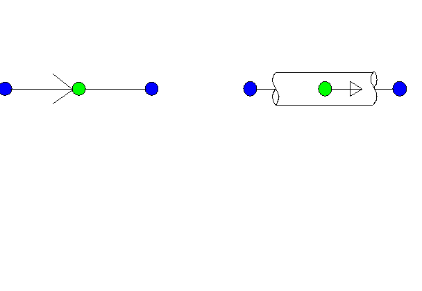
Fig. 4.18.1 Wanda Pipe component

Fall type

type label	description	active
Pipe	Pressurised pipe	No

As from the WANDA 4.0 release there is one pipe-model which includes all former pipe models. Although there are still two different symbols, the functionality is exactly the same.

4.18.1. Pressurised pipe

4.18.1.1. Mathematical model

The pipe can be considered the primary component in WANDA. The pipe is used to simulate the actual pressure wave propagation during transient simulations.

In steady state (Engineering Mode) dQ/dt = 0 and the pipe is considered as a fall type, modelled only by the following equation:

(4.18.1)\[H_{1}-H_{2}=\frac{f L Q^{2}}{2 g D A^{2}}\]

in which:

H1 ‑ H2	=	head loss from H‑node 1 to H‑node 2	[m]
Q	=	discharge through the pipe	[m3/s]
f	=	friction factor	[‑]
D	=	inner diameter	[m]
A	=	cross sectional area	[m2]

WANDA calculates the friction factor iteratively using the wall roughness or it can be directly specified by the user. Several friction models are included in WANDA, see “Friction models” on page 166 for details. Please note that the friction factor is only recalculated during the calculation if the Dynamic Friction is set to ‘Quasi-Steady’. With other friction models the friction factor is kept constant. For more details see “Wall roughness k-pipes” on page 168.

In Transient Mode the pipe model depends on the input property “Calculation mode”. If it is set to “waterhammer”, the PIPE is handled as a waterhammer pipe and the full waterhammer equations are solved. The wave propagation speed is calculated based on pipe and fluid properties. The user has also the option to specify the wave propagation speed according to his own needs. The waterhammer equations are given below, details about the wave propagation and the equations involved are discussed in Theory on waterhammer pipes in Chapter “General definitions” on page 149.

Momentum:

(4.18.2)\[\frac{1}{A_{\mathrm{f}}} \frac{\partial \mathrm{Q}}{\partial \mathrm{t}}+\mathrm{g} \frac{\partial \mathrm{H}}{\partial \mathrm{s}}+\frac{\mathrm{f} \mathrm{Q}|\mathrm{Q}|}{2 \mathrm{D} \mathrm{A}_{\mathrm{f}}^{2}}=0\]

Continuity:

(4.18.3)\[\frac{1}{c_{\mathrm{f}}^{2}} \frac{\partial \mathrm{H}}{\partial \mathrm{t}}+\frac{1}{\mathrm{~g} \mathrm{~A}_{\mathrm{f}}} \frac{\partial \mathrm{Q}}{\partial \mathrm{s}}=0\]

If the “calculation mode” is set to “rigid column”, the PIPE is considered as a pipe with infinite propagation speed. In a relatively short pipe the propagation speed can be regarded as infinite. Relatively short means smaller than the element length, ds, in which the compressible pipes are divided, such that the fluid velocity may be assumed constant (dv / ds = 0). In other words, the fluid in the pipe is regarded as incompressible. Hence, only the momentum equation is solved:

(4.18.4)\[H_{1}-H_{2}=\frac{L}{g A} \frac{d Q}{d t}+\frac{f L}{8 R g A^{2}} Q|Q|\]

in which:

Variable	Description	units
H1	upstream head	m
H2	downstream head	m
Q	discharge	m3/s
L	pipe length	m
D	Inner pipe diameter	m
A	cross sectional area	m2
R	hydraulic radius (A / P)	m
f	friction factor	‑

If the “calculation mode” is set to “Resistance”, the PIPE is considered as a hydraulic resistance. In this mode waterhammer phenomena and inertia are ignored, only the wall friction of the pipe is taken into account.

The flow number is a measure of the possibility of air transport through a downward sloping pipesection [3]. The flow number is calculated by the following equation:

(4.18.5)\[F=\frac{v}{\sqrt{g D}}\]

in which:

F	=	Flow number	[-]
v	=	velocity through the pipe	[m/s]
g	=	Acceleration due to gravity	[m/s2]
D	=	inner diameter	[m]

The pipe flow number is only calculated at steady state because the theory behind the flow number is based on steady state assumptions.

4.18.2. Pressurised pipe Properties

4.18.2.1. Cross section

The cross section of the pipe can be circular or rectangular. For rectangular cross sections, it is possible to define the size of the chamfers (filling of the corners, see Fig. 4.18.2) and their structural contribution. A larger chamfer and/or more structural contribution will increase the stiffness of the cross section, resulting in higher wave speed. A structural contribution of 0% means that the chamfers have no effect on the wave speed, whereas 100% gives full influence according to the theory as explained in section “Wave propagation speed” on page 173.

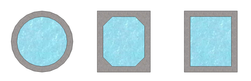
Fig. 4.18.2 Circular and rectangular cross section with and without chamfers.

4.18.2.2. Additional losses

If several local losses (like bends, Tee’s etc) exists in a pipe section, you may model them separately (pipe-resist-pipe-resist) or combine them in the pipe model. Combining them can be done in 2 different ways: using the ξ-annotation (single value or table) or the equivalent length annotation. For example:

for an elbow ξ_elbow is about 0.2

or

for an elbow L_eq is about 15 D

WANDA calculates the total resistance (friction and local losses) in the steady state and derives a combined friction factor that will be used during the unsteady state calculation. In the tables of the local losses the diameter of the local resistance may differ from the pipe diameter, but the combined friction factor will be related to the pipe diameter only. If the diameter of local loss differs from the main pipe, it can be specified in the column “Diameter”. If this column remains blank, the pipe diameter will be used.

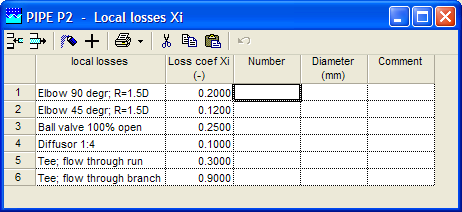
Fig. 4.18.3 Example of a table containing the local losses in a pipe section.

4.18.2.3. Geometry

Each PIPE must have a length input and height location. This so-called profile can be defined in several ways:

1. Scalar value for length

2. Length-height profile

3. Isometric layout specified with absolute XYZ co-ordinates

4. Isometric layout specified with differential XYZ co-ordinates.

Each type of profile input is translated to a longitudinal profile (X-H profile). In case of a scalar value the height of the beginning and the end of the pipe is derived directly from the adjacent H-nodes. The input height is the height of the centreline of the pipe, as indicated in figure 2 below.

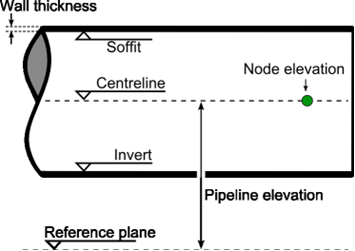
Fig. 4.18.4 Definition of the height of the pipe and the node elevation.

WANDA compares the input of the H-node height with the beginning and end of the Pipe. If there is a difference of more than half the pipe diameter, a warning is displayed in the property field “H-node height check”. Otherwise, “OK” is displayed.

Below an example of differential XYZ input based on the given isometric is given.

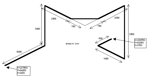
Fig. 4.18.5 PIPE isometric with differential input.

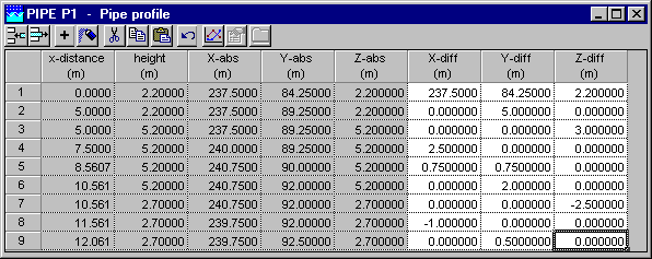
Fig. 4.18.6 Table of node locations for the PIPE isometric figure.

Please note the first row starts with the absolute XYZ coordinates followed by the differential coordinates.

The input is translated to real XYZ values and subsequently to a x-H profile. This x-H profile is shown in the location charts.

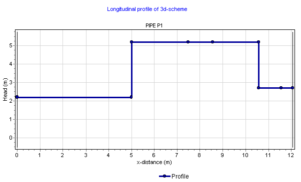
Fig. 4.18.7 Result of XYZ diff specified profile translated to x-H profile

It is not necessary that the pipe profile start with zero. Any positive value is possible. If you split a pipe into two parts (e.g. a VENT must be connected to the pipe) you only have to copy the pipe and delete the unnecessary rows.

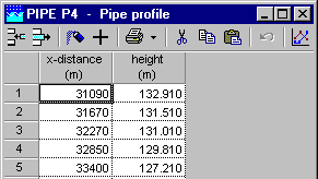
Fig. 4.18.8 The location chart (route) starts with the value specified in the first row of the table.

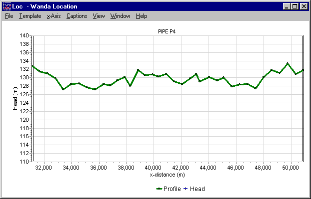
Fig. 4.18.9 Pipe profile starting with a non-zero begin location

4.18.2.4. Hydraulic specifications

description	input	unit	default	remarks
Cross section	Circle Rectangle	[-]	Circle
Inner diameter	real	[m]		if Cross section=Circle
Inner width	real	[m]		if Cross section=Rectangle
Inner height	real	[m]		if Cross section=Rectangle
Chamfer size	real	[m]	0	if Cross section=Rectangle
Chamfer structural contribution	real	[-]	0,67	if Cross section=Rectangle
Calculation mode	Waterhammer Rigid column Resistance		Waterhammer	Only in transient mode
Wave speed mode	Physical specified		Physical	if Calculation mode = Waterhammer
Wall thickness	real	[m]		if Wave speed mode = physical
Young’s modulus	real	[N/m2]		if Wave speed mode = physical
Specified wave speed	real	[m/s]		if Wave speed mode = specified
Friction model	D-W k D-W f H-W C-M	[ ]	D-W k	See “Friction models” on page 166
Wall roughness	real	[mm]		if Friction model = D-W k
Dynamic friction	Quasi-steady none			Only in transient mode and if Friction model = D-W k
Friction factor	real	[-]		if Friction model = D-W f
C coefficient	real	[-]		if Friction model = H-W
n coefficient	real	[-]		if Friction model = C-M
Additional losses	None Xi Xi-pos Xi-neg Xi table L_eq table	[-]	None
Local losses coeff	real	[-]		if Additional losses = Xi
Local losses pos. dir.	real	[-]		if Additional losses = Xi-pos Xi-neg
Local losses neg. dir	real	[-]		if Additional losses = Xi-pos Xi-neg
Local losses Xi	table			if Additional losses = Xi table
Local losses L_eq	table			if Additional losses = L_eq table
Geometry input	Length l-h xyz xyz diff	[-]
Length	real	[m]		if Geometry input = Length
Profile	table			if Geometry input = L-h, xyz or xyz diff
Upper limit pressure	real	[N/m2]		Only visible if checked in “Mode&options” window
Lower limit pressure	real	[N/m2]		Only visible if checked in “Mode&options” window
Location	real	[m]		If empty, chart button creates a location serie If filled in, chart button creates a time serie for nearest internal node

See also help on using the “Property Window” on page 43.

Remarks

The tables with local losses (Xi and L_eq tables) are derived from the tables as specified in the “Initial values” window (see menu/model). A local copy of this table is made and may be modified for this particular pipe. If you want to use other global settings for this case, first edit the “Initial values” tables before adding PIPE’s to the diagram.

The location charts of “Pressure” and “Head” shows the specified limits only if they are filled in. It is possible to specify these values after the simulation. If these fields are not visible, first check the “Upper/Lower limits in pipes” fields in the Mode & option window. You may change these values without re-calculating the case.

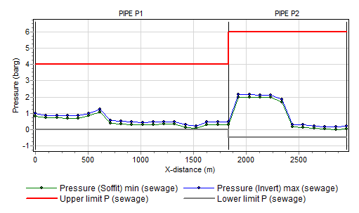
Fig. 4.18.10 Pressure location chart with additional pressure rating series

Note that the reference for the pressure output (centre line / soffit (top) / invert (bottom) is defined in the Mode & options window.

The main output properties like “Discharge” and “Pressure” contains vector based output (output values in each pipe node or element). That means that the chart button automatically creates a location chart. If you want a time chart in a particular pipe node you have to specify the location in the “Location” field.

To have direct access to the first and last node of the pipe (corresponding with the left and right H-node) you may extend the output property list with these points by checking the field “Connect point output in pipes”.

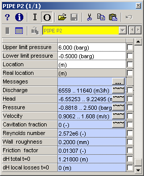
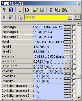
Figure 7: Two appearances of output properties window depending on Mode & Options setting “Connect point output in pipes”.

Pressing the chart button in these additional fields automatically generates a time series chart.

4.18.2.5. Component specific output

Output	Description
Pipe length [m]	Total pipe length based on entered profile
Wave speed [m/s]	Wave propagation speed based on fluid properties, pipe properties and time step
Pipe element count [-]	Amount of elements of same length in which pipe is divided.
Adapted wave speed [m/s]	Wave speed is adapted in such way that a integer number of elements (minimal 1) fits in the total length
Deviation adapted [%]	Ratio between wave speed and adapted wave speed. Must be less than 0.25 for a valid deviation
Cavitation fraction [-]	Ratio between cavitation volume and element volume Must be less than 0.20 for valid range of cavitation algorithm
H-node height check	Input validation between H-node height with corresponding pipe node elevation. OK means the difference is less than 0,5 D, otherwise “Warning” is displayed.
Wall roughness	The wall roughness based on the friction factor and including local losses
dH total t= 0	Total head losses across the pipe at steady state
dH local losses t=0	Head loss due to local losses at steady state
Flow number at t=0	The flow number at steady state

4.18.2.6. H-actions

None

4.18.2.7. Example

None