4.25. Resistance

4.25.1. RESIST (class)

Fig. 4.25.1 Local resistance or loss

Fall type

type label	Description	active
Resist quadr. xi	Dimensionless -value from loss equation	No
Resist quadr. C	-value from loss equation	No
Resist linear C	-value from loss equation \(\Delta H=C Q\)	No
Resist quadr. Initial Q	Initial is specified, from loss equation is computed.	No
Resist 2-way quadr.xi	Dimensionless -value from loss equation -value depends on flow direction	No
Resistance polynomial	Resistance according user-defined polynomial	No

4.25.1.1. Mathematical model

A resistance is modelled by the following equations:

(4.25.1)\[H_{1}-H_{2}=a \xi Q_{1}\left|Q_{1}\right|\]

in which:

Variable	Description	Units
H1	Upstream head	[m]
H2	Downstream head	[m]
a	\(1 /\left(2 g A_{\mathrm{r}}^{2}\right)\)	[s2/m5]
ξ	loss coefficient	[‑]
Q1	discharge through RESIST	[m3/s]
Ar	discharge area resistance	[m2]

The discharge area does not have to be equal to the area of the adjacent pipes.

The area is calculated from the resistance diameter D_r according to

(4.25.2)\[A_{\mathrm{r}}=\pi D_{r}^{2} / 4\]

Tip:

The RESIST can be used to model all kinds of resistant components without a relevant length, e.g.:

• A number of bends

• Entrance, exit losses

• Filters

• Heat exchangers, etc.

4.25.2. Resist quadr. xi

4.25.2.1. Hydraulic specifications

Description	input	unit	range	default	remarks
inner diam­eter	real	[m]	(0-5]
loss coeffi­cient	real	[-]	[0-100]

See also “Mathematical model” (Section 4.25.1.1).

4.25.2.2. Component specific output

None

4.25.2.3. H-actions

None

4.25.2.4. Component messages

None

4.25.3. Resist quadr. C

4.25.3.1. Hydraulic specifications

description	input	Unit	range	default	remarks
C-value (∆H=CQ2)	real	[s2/m5]	[0-100]

See also “Mathematical model” (Section 4.25.1.1).

4.25.3.2. Component specific output

None

4.25.3.3. H-actions

None

4.25.3.4. Component messages

None

4.25.4. Resist linear C

4.25.4.1. Hydraulic specifications

description	input	unit	range	default	remarks
linear C-value	real	[s/m2]	[0-100]
(­∆H=CQ)

See also “Mathematical model” (Section 4.25.1.1).

4.25.4.2. Component specific output

None

4.25.4.3. H-actions

None

4.25.4.4. Component messages

None

4.25.5. Resist quadr. Initial Q

4.25.5.1. Hydraulic specifications

description	input	unit	range	default	remarks
initial discharge	real	[m3/s]	(0-10]

See also “Mathematical model” (Section 4.25.1.1).

4.25.5.2. Component specific output

None

4.25.5.3. H-actions

None

4.25.5.4. Component messages

Message	Type	Explanation
C‑value (resistance) = … [s2/m5]	Info

4.25.6. Resist 2-way quadr.xi

4.25.6.1. Hydraulic specifications

Description	input	unit	range	default	remarks
inner diam­eter pos flow	real	[m]	(0-5]
inner diameter neg flow	real	[m]	(0-5]
loss coeff. pos flow (xi+)	real	[-]	[0-100]
loss coeff. new flow (xi-)	real	[-]	[0-100]

4.25.6.2. Component specific output

None

4.25.6.3. H-actions

None

4.25.6.4. Component messages

None

4.25.7. Resistance polynomial

Fig. 4.25.2 Polynomial resistance

Fall type

type label	description	active
Resistance polynomial	Resistance described by second order polynomial	no

4.25.7.1. Mathematical model

The resistance of a particular hydraulic object is mostly a non-linear function. If field measurements are carried out, the pressure head difference and related discharge can be shown in a chart, see figure below.

[CHART]

The function of this resistance can be described by a second order polynomial:

• \(\Delta H=a+b Q+c Q|Q|\) (1)

in which:

• ∆H = pressure drop H1-H2 [m]

• Q = Discharge through resist [m³/s]

• a,b,c = coefficients [-]

• H1 = upstream pressure head [m]

• H2 = downstream pressure head [m]

The coefficients a, b, and c can be derived e.g. using EXCEL (insert trendline). The coefficient a is the static pressure head.

In the figure below, the derived function together with the measured points are drawn. Note that the coefficients are based on SI-units.

[CHART]

Remark:

The polynomial is valid for positive and negative flow.

Note that the coefficient “A” is a constant head loss and is only valid for a positive flow direction. That means that with a negative flow, the headloss contribution “A” (defined as H1-H2) is the same as for positive flow.

4.25.7.2. Hydraulic specifications

Description	input	unit	range	default	remarks
Coefficient a in ∆H=a+bQ+cQ|Q|	real	[-]	(-108 -108)
Coefficient b in ∆H=a+bQ+ cQ|Q	real	[-]	(-108 -108)
Coefficient c in ∆H=a+bQ+ cQ|Q	real	[-]	(-108 -108)

4.25.7.3. Component specific output

None

4.25.7.4. H-actions

None

4.25.7.5. Component messages

None

4.25.7.6. Example

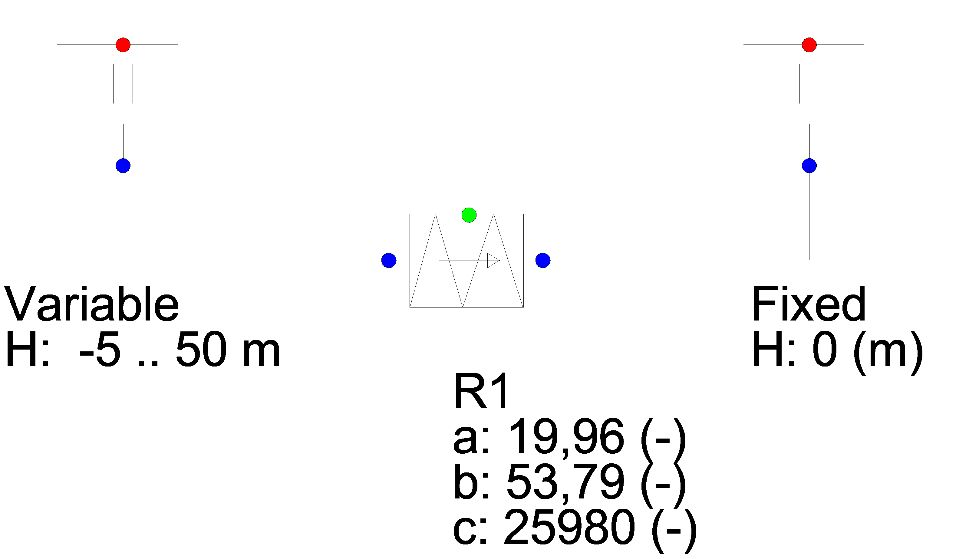
Fig. 4.25.3 Schematic overview of the wanda model

The level in the upstream reservoir varies from 50 m to -5 m; the level in the downstream reservoir remains constant at H= 0 m.

Next figure shows the discharge and level as functions of time.

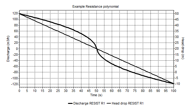
Fig. 4.25.4 Pressure as function of time for a polynomial resist.

The next chart shows the pressure head ΔH related to the discharge Q. The WANDA results are exactly the same as the theoretical polynomial.

[CHART]