4.36. Vent, Air valve with filling pipe section

4.36.1. VENT2LEG (class)

Fig. 4.36.1 Fall type

type label	description	active
vent2leg	Vent with automatic in/outflow. Capacity specified with discharge coefficients. The level effect is automatically taken into account based on the profile of the pipelines connected to the vent	No

4.36.1.1. Mathematical model

The vent or air valve is a component through which air can enter into or be expelled from the hydraulic system. This is usually achieved by a floating-ball valve mechanism (figures 1, 2 and 3). The purpose of the vent is to prevent cavitation or intolerable underpressures.

Figure 1: In/outlet vent in air inlet status	Figure 2: In/outlet vent in air outlet status

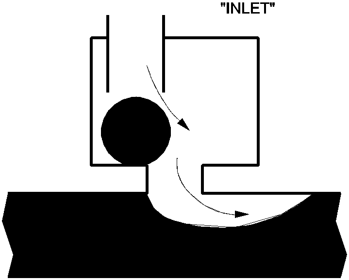
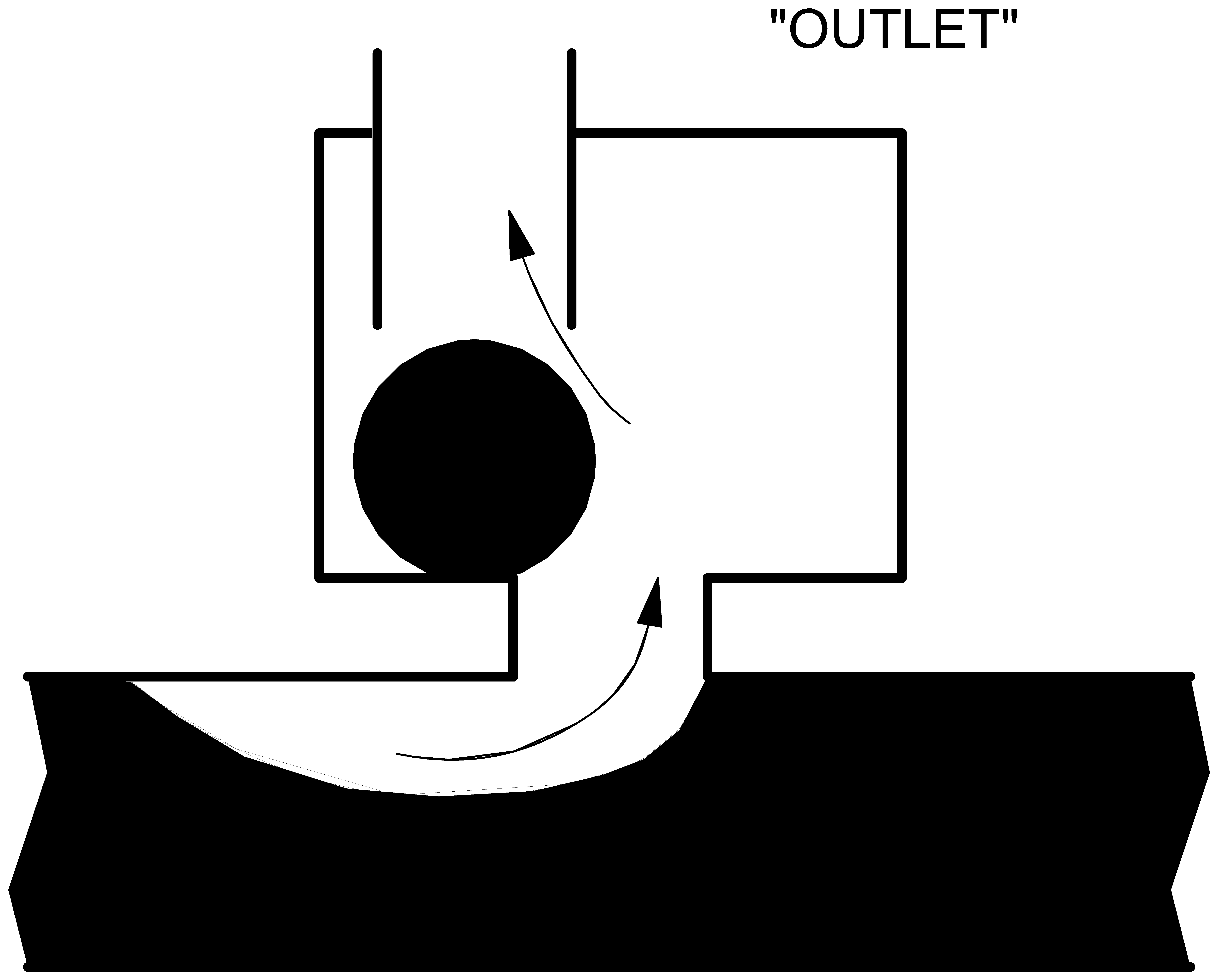
If the internal pressure head in the system drops below the elevation of the vent, the floating-ball valve opens and air can enter the system (Figure 1). The air entering the system will expand due to the internal pressure being lower than atmospheric pressure. If the air remains in the vicinity of the vent (e.g. in case the vent is located at a “high” point in the system) it will be expelled through the same vent if the internal pressure rises again above the elevation of the vent (Figure 2). Meanwhile the air will also be compressed due to the internal pressure being higher than atmospheric. The vent closes at the instant the amount of air is smaller than the residual air volume (Figure 3).

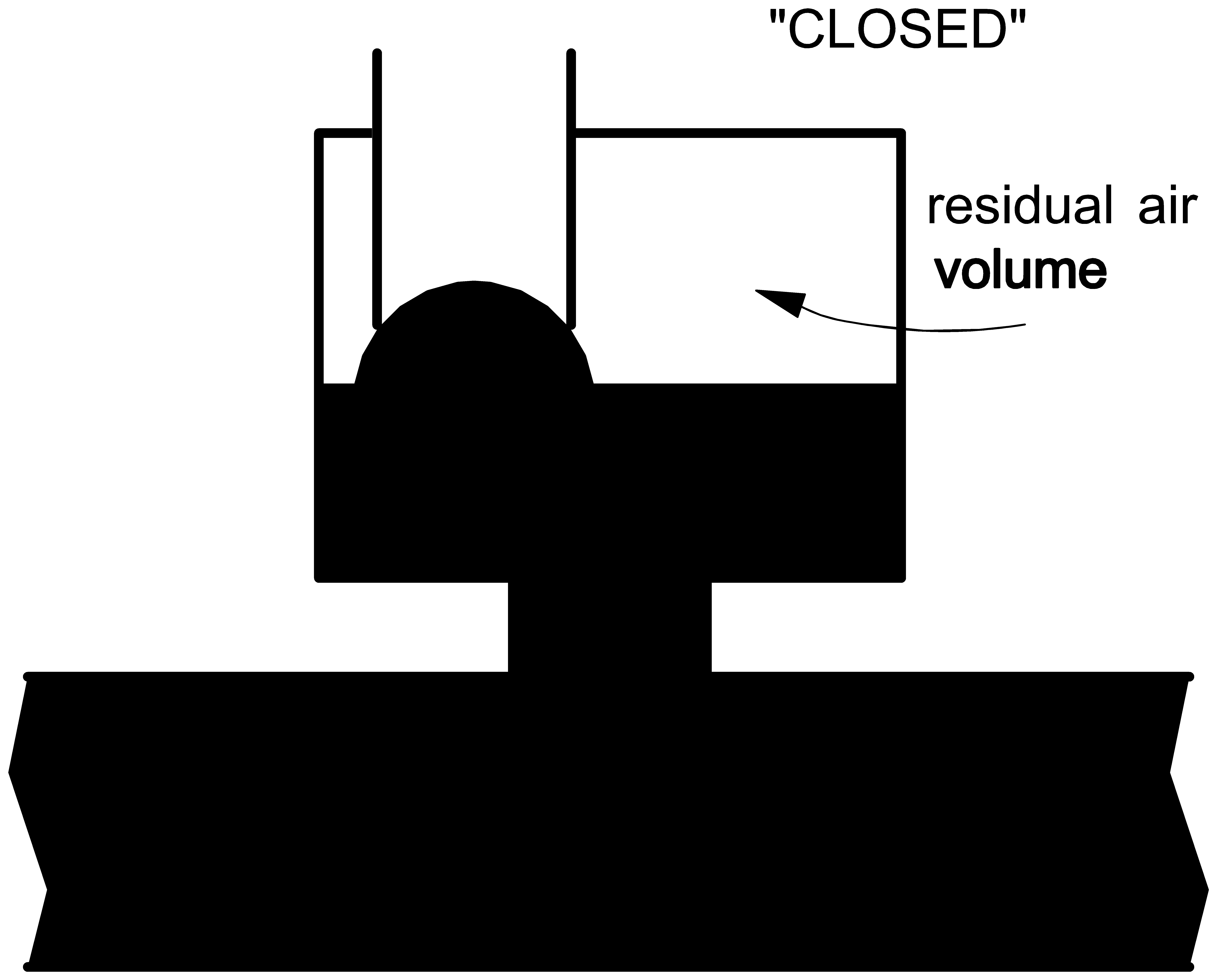
Fig. 4.36.2 In/outlet vent in closed status

The air flow is compressible, with the consequence that due to local occurrence of supersonic velocities and shock waves, choking flow may arise. The air inlet capacity is therefore truncated to a certain level. If the internal pressure reduces below this level, the air flow does not increase anymore. The expansion and compression of the air may be isothermal, adiabatic or polytrophic. Since Wanda is not a two-phase flow computer code, it is not capable of describing the entrainment and transportation of air in the pipeline as such. The calculations are performed under the assumption that air is not transported into the pipeline. A warning is included when this assumption is no longer valid. This check is based upon the value of the flow number. For more information see Ref. [1] and Ref. [2].

The vent model is merely a boundary condition describing a pressure-discharge relation. In reality, the amount of liquid within the system decreases when air enters the system. the compressibility of the air is taken into account in the discharge supplied by the vent to the system. The vent component supplies liquid to the system and therefore an error in the momentum balance (inertia forces) will be introduced. This error is small, if the amount of air is small compared to the pipeline volume. The continuity balance is not violated.

Changing water levels due to air entrainment or expansion/compression is automatically taken into account based on the profile of the connecting pipes. As the volume of air increases, the fluid level drops accordingly.

For the description of the mathematical model two states are defined:

• Closed air valve,

• Open air valve

In case of “closed-in” air (state 1) the component behaves like an air vessel:

(4.36.1)\[P_{a i r} V_{a i r}^{k}=C\]

in which:

Pair	=	absolute air pressure on fluid level	[Pa]
Vair	=	air volume	[m3]
k	=	Laplace coefficient (ratio of specific heats)	[-]
C	=	Constant	[J]

The second equation is the continuity equation, which states that the change of volume in air is equal to the in- and outflow of the vent to both connecting nodes.

(4.36.2)\[Q_{1}-Q_{2}+\left(\frac{P_{a t n}}{P_{\text {air }}}\right)^{\frac{1}{k}} Q_{\text {air }}=0\]

in which:

Q1	=	Discharge at connection point 1	[m3/s]
Q2	=	Discharge at connection point 2	[m3/s]
Patm	=	Atmospheric pressure	[Pa]
Qair	=	Air flow rate at atmospheric pressure and temperature	[Nm3/s]

During the closed state the change of volume of air is due to compression and expansion of the air.

The third equation is an equation equalling the air pressure on both sides of the vent.

The air pressure is given by:

(4.36.3)\[P=P_{a t m}+\rho g\left(H_{i}-w_{i}\right)\]

in which:

P	=	Absolute air pressure on fluid level	[Pa]
ρ	=	Density of the fluid	[kg/m3]
g	=	Gravitational acceleration	[m/s2]
H	=	Head at ith connection point	[m]
w	=	Fluid level at ith connection point	[m]

Since the air pressure on both sides of the vent is equal, this equation becomes:

(4.36.4)\[H_{1}-H_{2}=w_{1}-w_{2}\]

In the open state (2) the change of air volume in time is dependent of two phenomena:

1. The compression/expansion of the air.

2. The amount of air leaving/entering the system.

The former is handled in the same way as with state 1 (closed). The latter is determined by formula (5) to (8). Based on the air pressure the direction of the air flow is automatically determined.

Vent capacity (defined by coefficients)

The following formulae are based on Ref. [3].

1. Subsonic air flow in

(4.36.5)\[Q_{a i r}=C_{i n} A_{\text {in }} \sqrt{7 R T_{0}} \sqrt{\left(\frac{P}{P_{\text {atm }}}\right)^{1.4286}-\left(\frac{P}{P_{a t m}}\right)^{1.714}} ; P_{a t m}>P>0.53 P_{\text {atm }}\]

in which:

Ain	=	inlet area	[m2]
Cin	=	inlet discharge coefficient	[-]
R	=	gas constant	[J/kg⋅K]
T0	=	ambient air temperature	[K]

2. Critical flow in

(4.36.6)\[Q_{\text {air }}=C_{\text {in }} A_{\text {in }} \sqrt{7 R T_{0}} 0.259 ; P<0.53 P_{\text {atm }}\]

3. Subsonic air flow out

(4.36.7)\[Q_{\text {air }}=-C_{\text {out }} A_{\text {out }} \sqrt{7 R T_{0}}\left(\frac{P}{P_{a t m}}\right)^{\frac{k+1}{2 k}} \sqrt{\left(\frac{P_{a t m}}{P}\right)^{1.4286}-\left(\frac{P_{a t m}}{P}\right)^{1.714}} ; \frac{P_{a t m}}{0.53}>P>P_{a t m}\]

in which:

Aout	=	outlet area	[m2]
Cout	=	outlet discharge coefficient	[-]

4. Critical flow out

(4.36.8)\[Q_{\text {air }}=-C_{\text {out }} A_{\text {out }} \sqrt{7 R T_{0}}\left(\frac{P}{P_{\text {atm }}}\right)^{\frac{k+1}{2 k}} 0.259 ; \frac{P_{\text {atm }}}{0.53}<P\]

Level effect

The level effect is automatically included based upon the pipe profile of pipes directly connecting to the 2-leg air valve. It is therefore only possible to connect one pipe to each side of the air valve and no other components. A connection pipe between the air valve and the pipeline can be included by specifying its diameter and height, see Figure 4. For the level effect an engineering approach is used to calculate the volume in bends. Since the most important result is the expelling of the last air, this approximation is acceptable. The dynamic behaviour of the water levels in both legs depends on the actual water levels relative to the bottom elevation. If we denote the local pipe bottom elevation with b, then the following states are feasible:

\(w_1\)	\(w_2\)	Description	Applicable equations
\(>b\)	\(>b\)	both levels are identical.	\(w_{1}=w_{2}\) and \(Q_{1}-Q_{2}=A_{1}\left(w_{1}\right) \frac{d w_{1}}{d t}+A_{2}\left(w_{2}\right) \frac{d w_{2}}{d t}\)
\(=b\)	\(<b\)	leg 1 fills leg 2, if \(Q_1 > 0\)	\(w_{1}=b\) and \(Q_1-Q_2 = A_2(w_2)\frac{d w_2}{dt}\)
\(<b\)	\(=b\)	leg 2 fills leg 1, if \(Q_2 < 0\)	\(w_{2}=b\) and \(Q_1-Q_2 = A_1(w_1)\frac{d w_1}{dt}\)
\(Mb\)	\(<b\)	system is fully decoupled	\(Q_1 = A_1 w_1 \frac{d w_1}{dt}\) and \(Q_2 = A_2 w_2 \frac{d w_2}{dt}\)

The fact that the water level remains equal to the local bottom elevation implies that the overflow is idealised.

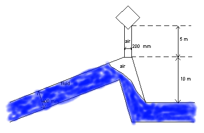
Fig. 4.36.3 Example of 2-leg air valve with standpipe

Air transport

Wanda is a single phase simulation tool, thus air transport through pipelines is not included. The air valve model can be used for all processes (such as slow filling) where air is expelled or taken in at the same air valve where air is not transported through the pipeline. Air is partially transported when the flow number is greater than 0.6: If the flow number is greater than 0.9 all air is transported. The flow number is given by:

(4.36.9)\[F r=\frac{v}{\sqrt{g D}}\]

in which:

Fr	=	Flow number	[-]
v	=	Flow velocity	[m/s]
D	=	Pipe diameter	[m]

A warning is given when one of these criteria is exceeded. Note that simulation results are invalid if the flow number exceeds 0.6. For more background see Ref. [1] and Ref. [2].

4.36.2. VENT2LEG properties

4.36.2.1. Hydraulic specifications

description	Input	unit	range	default	remarks
Height connection pipe	Real	[m]
Diameter connection pipe	Real	[m]
Laplace coefficient	Real	[-]	[1-1.4]
Ambient air temperature	Real	[°C]
Inlet discharge coefficient	Real	[-]	[0-1]		See remark
Outlet discharge coefficient	Real	[-]	[0-1]		See remark
Inlet discharge area	Real	[m2]	≥0
Outlet discharge area	Real	[m2]	≥0
Delta P for open	Real	[Pa]
Residual air volume	Real	[m3]	[0-1]
Initial state	Closed Open			Closed
Initial upstream fluid level	Real	[m]
Initial downstream fluid level	Real	[m]

See also “Mathematical model” on page 450.

Remark

Please be aware that for deriving the discharge coefficients C_in and C_out from a K_v-value (m³/h if = 1 bar), the manufacturer most probably specifies the capacity in atmospheric cubic metres per second. In general, the discharge coefficients describe the amount of contraction of the air flow through the orifices and will probably be in the range of 0.5 to 1.0.

To simulate an air valve, which only lets air into the system the outlet discharge coefficient can be set to 0, in the same way an outlet air valve can be modelled by setting the inlet discharge coefficient to zero.

Important Notice: In case of vents with large capacity it is well possible to have a very sensitive computation in which small pressure differences cause large air flows and volumetric effects. Although the program is optimised to find the most accurate solution, numerical oscillations may still occur (inertia is not taken into account). In that case it is up to the user to adjust (reduce) the time step and the convergence criteria to reduce the oscillations.

See also “Mathematical model” on page 450.

4.36.2.2. Component specific output

Air volume [m³]

Air flow [m³/s]

Air pressure (absolute) [N/m².abs]

Fluid level 1 [m]

Fluid level 2 [m]

Flow number [ ]

4.36.2.3. H-actions

None

4.36.2.4. Component messages

Message	Type	Explanation
Not exactly one pipe connected to connection point i	Error
Initial upstream fluid level above air valve top	Error
Initial downstream fluid level above air valve top	Error
Initial upstream fluid level above pipe bottom high point and initial downstream fluid level below pipe bottom high point	Error
Initial downstream fluid level below pipe bottom high point and initial upstream fluid level above pipe bottom high point	Error
Starts in open phase	Error
Air valve opens	Info
Air valve closes	Info
Air is transported	Warning
All air is transported	Warning
Pipeline drained below local bottom point on side 1, results physically invalid	Warning	The level in the pipe upstream has dropped to below the lowest allowable draining level (local low point). Further lowering of the level is not computed and the level will act as a boundH, not further reducing the flow.*
Pipeline drained below local bottom point on side 2, results physically invalid	Warning	The level in the pipe downstream has dropped to below the lowest allowable draining level (local low point). Further lowering of the level is not computed and the level will act as a boundH, not further reducing the flow.*

* These messages may occur if the pipeline elevation does not extend to below the head condition at the other side. E.g. the emptying of the pipe towards the downstream side can then not be carried on until the level of the downstream boundH.

References

[1] Pothof, I.W.M., Co-currunt air-water flow in downward sloping pipes, 2011, ISBN: 978-90-89577-018-5

[2] Tukker, M.J., Kooi, C, Pothof, I. (2013): Hydraulic design and management of wastewater transport systems, CAPWAT Manual, published by IOS Press BV, Netherlands, http://capwat.deltares.nl

[3] Streeter, V.L., Wylie, E.B., 1978: Fluid Transients. McGraw-Hill, New York.