4.2. Modular concept of H-component properties

In the property window all input and output properties are displayed. The property window can be divided in 5 parts:

Table 4.2.1 Components defined in the property window.

Type	Description
General input data	Name, comment, keywords etc
Component specific input data	Type dependent
Action table	Type dependent for active types only (H-actions)
General output data	Messages, Pressure, Head, Discharge and Velocity
Component specific output data	Type dependent

The visibility of some properties can be managed using the checkboxes in the upper part of the Mode & Options window in the “Model”| menu.

The type dependent properties are described separately for each component type. Some details about the action table are described in next chapter.

4.2.1. Specify actions

Hydraulic transients in a piping system are caused by changes in the flow conditions. These changes are initiated by manoeuvring H‑components in the system, called actions. Not all components in a pipeline system can be activated. A component is categorised as either an active or a passive component, depending on its abilities.

An action is described using a control parameter specified as a function of time. The controlable parameter varies by component. g198

Notes

1. The interpretation of an action into an action table is illustrated below using the example of a control valve. Note that values of the control parame­ter at times between two successive points in the action table are obtained using linear interpolation.

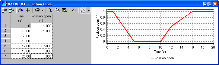
Fig. 4.2.1 The example shows the linear interpolation of action table values for a control valve

The valve is fully open at t = 0 s;

• it begins to close at a constant rate;

• the closure is complete after 5 s;

• it remains closed until t = 10 s;

It turns open again

• the opening rate is slower between t = 12 s and t = 16 s;

• the valve is fully open after 16 s;

• the valve remains open until the end of the computation;

2. Sudden actions can be modelled by reducing the time steps in the action table to one calculation time step. If necessary the calculation time step should be reduced.

Example

The following action table describes that the valve is open at t = 0 s. It is suddenly closed at t = 1.0 s, remains closed for 5 seconds, then suddenly opens and remains open until t = 20.0 s.

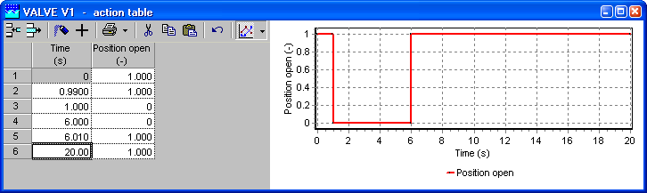
Fig. 4.2.2 Example of a valve closure defined with an action table.

Theoretically, a mathematical step-function can be used to describe an instantaneous action, for example, the instantaneous closure of a valve. However, such an action is unrealistic as it always takes some time in practice. The approximation above is more realistic than a mathematical step-function.

3. The last point in the action table is not necessarily the end time of the computation. WANDA uses the last entry in the table and assumes it does not change until the end of computation. Consequently the last entry in the table above may be removed.