4.20. Pump

4.20.1. PUMP (class)

Fig. 4.20.1 Wanda pump component

Pump

Fall type

type label	description	active
Pump	Complete pump model with various data and drives. Positive and negative speeds	yes

4.20.1.1. Mathematical model

In the most general case a pump can operate in four QH-quadrants for \(N≥0\) and in four \(QH\)-quad­rants for \(N<0\). In WANDA, two pump models are distinguished: the pump model limited to the \(N≥0\) case (section 4.23.1.2) and the complete pump model for all \(N (<0, =0\) and \(>0)\), see section 4.23.1.3.

Basic equations

The running pump is characterised by the following functions in the first quadrant for \(N>0\):

(4.20.1)\[ H=f(Q), N=N_{r}\]

(4.20.2)\[E = f(Q), N = N_r\]

in which:

\(H\)	pump head	m
\(Q\)	pump discharge	m3/s
\(E\)	pump efficiency	-
\(N\)	pump speed	rpm
\(N_r\)	rated pump speed (at which the functions f and g are specified)	rpm

To describe a tripping pump the torque function must be known as well:

(4.20.3)\[ T=f(Q), N=N_{r}\]

To derive the functions (4.20.1), (4.20.2) and (4.20.3) for other pump speeds \(N_i\) than the rated pump speed \(N_r\) the affinity rules are used:

(4.20.4)\[\frac{H(N_i)}{H(N_r)} = \left( \frac{N_i}{N_r} \right)^2\]

(4.20.5)\[\frac{Q(N_i)}{Q(N_r)} = \frac{N_i}{N_r}\]

(4.20.6)\[\frac{T(N_i)}{T(N_r)} = \left( \frac{N_i}{N_r} \right)^2\]

The affinity rules – also known as the homologous relations – are based on the assumption that the flow field and the accompanying pressure field are independent of the size of the pump as long as the shape (proportions) remain the same, and that also the efficiency does not change with the size of the pump.

To simulate a tripping pump Newton’s second law is used in terms of rotating mass:

(4.20.7)\[T_{d}-T=I_{p} \frac{d N}{d t} \frac{2 \pi}{60}\]

in which \(T_d\) is the driving torque and \(T\) is the torque exerted by the fluid on the pump impeller. \(I_p\) denotes the polar mass moment of inertia [kgm2] of rotating mass (=motor + impeller + fluid). Note: sometimes the value \(GD^2\) (GeeDeeSquared) is used which is four times the \(I_p\).

In normal running operation \(T_d = T\) and the pump will run at a steady speed. Due to e.g. power failure, \(T_d = 0\), and therefore during pump trip the decaying pump speed can be calculated from:

(4.20.8)\[dN = - \frac{60}{2 \pi} \frac{T}{I_p} dt\]

In the procedure this differential equation is solved using Euler’s method. The torque for \(N_i\) is calculated using the affinity rules (4). In the case of a starting pump, \(T_d\) is deter­mined by the speed-torque relation (in tabular form) of the driving motor-gearbox combination.

4.20.1.2. The pump model for N≥0 (QHE table)

The equations describing the discharge (eq. (6.13.2)) and the efficiency (eq. (6.13.3)) are usually unknown in algebraic form. A pump manufacturer normally provides the discharge (eq. (6.13.2)) and efficiency (eq. (6.13.3)) curves in a graphical form, which only specify the first quadrant for \(N = N_r\). The graphical curves need to be transforemd to tables, such that at the start of the simulation the \(QH\) table and the \(QE\) table are known for \(N_r\). The torque table can be derived using:

(4.20.9)\[T = \frac{\rho_f g Q H}{\eta N_r}\]

with:

Variable	Description	Units
\(T\)	Pump torque (shaft)	Nm
\(\rho_f\)	Fluid density	kg/m3
\(Q\)	Pump dishcarge	m3/s
\(H\)	Pump head	m
\(\eta\)	Pump efficiency	-
\(g\)	Gravitational acceleration	m/s2
\(N_r\)	Rated pump speed (i.e., where the f and g curves have been defined)	rpm

However, the functions \(H\) and \(T\) have to be known in the second and fourth quadrant to simulate a pump trip. To get the values outside the table range the tables are extended to the ‘left hand’ and ‘right hand’ side with so-called extrapolation parab­olas. These parabolas have the following general forms:

\(QH\), right of the table range:

(4.20.10)\[\frac{H}{H_r} = A_H \left( \frac{Q}{Q_r} \right)^2 + B_H \left( \frac{Q}{Q_r} \right) + C_H\]

\(QH\), left of the table range:

(4.20.11)\[\frac{H}{H_r} = D_H \left( \frac{Q}{Q_r} \right)^2 + E_H \left( \frac{Q}{Q_r} \right) + F_H\]

\(QT\), right of the table range:

(4.20.12)\[\frac{T}{T_r} = A_T \left( \frac{Q}{Q_r} \right)^2 + B_T \left( \frac{Q}{Q_r} \right) + C_T\]

\(QT\), left of the table range:

(4.20.13)\[\frac{T}{T_r} = D_T \left( \frac{Q}{Q_r} \right)^2 + E_T \left( \frac{Q}{Q_r} \right) + F_T\]

The parabolas are defined in dimensionless form, by dividing the \(H\), \(T\) and \(Q\) curves with their rated values to \(H_r\), \(T_r\) and \(Q_r\) (i.e. the values in the maximum efficiency point at the rated pump speed \(N_r\)). The extrapolation coefficients \(A\) and \(D\) are derived in from empirical data as a function of the pump specific speed \(N_s\) (see table 1 to 4).

Table 1: A_H coefficients and derivatives versus the pump specific speed NS

\(N_s\)	\(A_H\)	\(dA_H/dN_S\)
10	-0.446	-0.004100
20	-0.487	-0.005075
50	-0.649	-0.007263
100	-1.068	-0.009730
150	-1.622	-0.008070
200	-1.875	0.004690
250	-1.153	0.014440

Table 2: D_H coefficients and derivatives versus the pump specific speed NS

\(N_s\)	\(D_H\)	\(dD_H/dN_S\)
10	0.566	0.005100
20	0.617	0.006400
50	0.822	0.009650
100	1.389	0.013480
150	2.170	0.007370
200	2.126	-0.009100
250	1.260	-0.017320

Table 3: A_T coefficients and derivatives versus the pump specific speed NS

\(N_s\)	\(A_T\)	\(dA_T/dN_S\)
10	-0.332	-0.003800
20	-0.370	-0.004675
50	-0.519	-0.007588
100	-0.977	-0.010660
150	-1.585	-0.006080
200	-1.585	0.008050
250	-0.780	0.016100

Table 4: D_T coefficients and derivatives versus the pump specific speed \(N_s\)

\(N_s\)	\(A_T\)	\(dD_T/dN_S\)
10	0.704	0.005800
20	0.762	0.007375
50	0.999	0.010050
100	1.566	0.011270
150	2.126	0.002140
200	1.780	-0.013450
250	0.781	-0.019980

The specific speed (\(N_s\)) of a pump is used to characteriste its type and is defined as:

(4.20.14)\[N_s = \frac{N_r\sqrt{Q_r}}{{H_r}^{3/4}}\]

Low values (<50) indicate a centrifugal (or radial) type of pump and high values (>200) indicate an axial type of pump. Each pump has a specific \(N_s\), which usually is not equal to one of the tabulated values of \(N_s\). Linear interpolation is used to obtain the values for each \(N_s\) as:

(4.20.15)\[A_H(N_{spec}) = A_H(N_s) + (N_{spec} - N_s) \frac{dA_H}{dN_s}\]

The same method is applied for the other empirical coefficients (i.e., \(D_H\), \(A_T\) and \(D_T\)). The remaining coefficients are determined as follows:

• \(B_H\) and \(C_H\) are calculated using the last two \(QH\) table points.

• \(E_H\) and \(F_H\) are calculated using the first two \(QH\) table points.

• \(E_T\) and \(F_T\) are calculated using the first two \(QT\) table points.

The \(B_T\) and \(C_T\) coefficients are determined with the following steps:

A. First, the intersection point between the \(\frac{H}{H_r}\) curve and the \(T = 0\) line is determined:

(4.20.16)\[\frac{H}{H_r} = A_H\left(\frac{Q}{Q_r}\right)^2 + C_H\]

(4.20.17)\[\frac{H}{H_r} = \phi \left(\frac{Q}{Q_r} \right)^2 \ \text{, at the } T = 0 \ \text{line}\]

The \(T = 0\) line describes the relation between \(H\) and \(Q\) when the pump speed is such that the pump exactly maintains a hydraulic torque \(T = 0\). The coefficient \(\phi\) = -0.3 is an empirically derived coefficient, which is assumed to be a constant and independent of the pump specific speed. However, the coefficient \(\phi\) varies in reality between about -0.1 and -0.4. The intersection of both curves defines the discharge \(Q_{T0}\) for which \(T = 0\).

B. \(B_T\) and \(C_T\) are determined from the last table point of the \(QT\) table and the discharge \(Q = Q_{T0}\) for which \(T = 0\).

Figure 1 shows an example of the extrapolation parabolas where \(Q_{T0} = 3.52\) (dimensionless!).

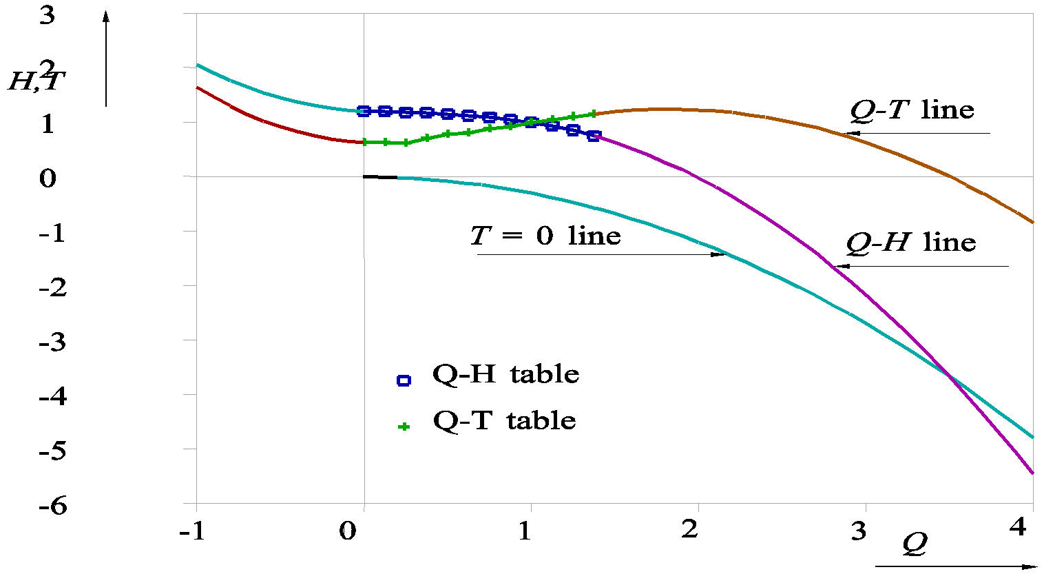
Fig. 4.20.2 Dimensionless curves of pump for \(N>0\)

4.20.1.3. The complete pump model

In order to obtain the pump function for positive and negative flow as well as positive and negative pump speed, heads and torque’s for all combinations of \(Q\) and \(N\) have to be measured and plotted as isolines in an N-Q graph. This has been carried out for a number of pumps in literature. These pumps are of varying type (radial flow, mixed flow, axial flow) denoted by specific speeds of 25, 147 and 261 (SI units) respectively (see Wylie, Fluid Transients in Systems, 1993).

It has proven convenient to use dimensionless quantities for head, torque, discharge and speed, by dividing the quantities by their respective values at rated \((r)\) conditions.

(4.20.18)\[h=\frac{H}{H_{r}} ; \quad \beta=\frac{T}{T_{r}} ; \quad q=\frac{Q}{Q_{r}} ; \quad \alpha=\frac{N}{N_{r}}\]

Expressed in these dimensionless quantities the affinity laws read:

(4.20.19)\[\frac{h}{\alpha^{2}} \text { vs. } \frac{q}{\alpha} \quad \frac{\beta}{\alpha^{2}} \text { vs. } \frac{q}{\alpha} \quad \frac{h}{q^{2}} \text { vs. } \frac{\alpha}{q} \quad \frac{\beta}{q^{2}} \text { vs. } \frac{\alpha}{q}\]

From a computational viewpoint, these relations are difficult to handle (dividing by zero when pump speed passes zero, and changing signs during transients). Marchand and Suter have overcome this difficulty by using:

(4.20.20)\[W H=\frac{h}{\alpha^{2}+q^{2}} \text { vs. } \tan ^{-1} \frac{q}{\alpha} \quad \text { and } \quad W B=\frac{\beta}{\alpha^{2}+q^{2}} \text { vs. } \tan ^{-1} \frac{q}{\alpha}\]

For complete pump data in all zones of operation, a polar diagram of \(\tan ^{-1} \frac{q}{\alpha}\) vs. WH and \(\tan ^{-1} \frac{q}{\alpha}\) vs. WB can be plotted as closed curves. This is usually done in the form of a rectangular plot (see figure 2) in which the abscissa \(x = 2\pi (=\tan ^{-1} \frac{q}{\alpha}\) ). The addition of \(\pi\) is intended to have only positive values for \(x\) (ranging from 0 to 2).

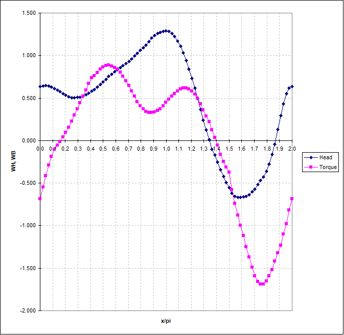
Fig. 4.20.3 Dimensionless Suter curves of radial pump (N_S=25, SI units)

These curves can for any \(\alpha\) be transformed into head and torque as functions of discharge and made dimensional by substitution of actual values in (12) and (14). An example transformed from figure 2 is given in figure 3.

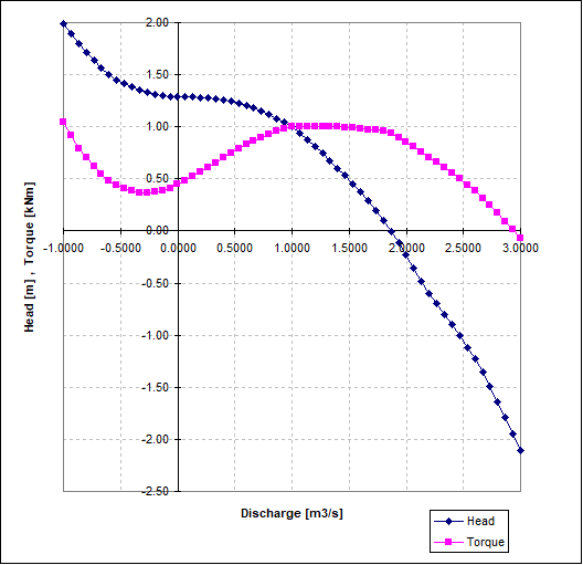
Fig. 4.20.4 Dimensionless curves of pump for \(N>0\)

This procedure works equally well for \(\alpha < 0 , \alpha = 0\) and \(\alpha > 0\). The user input consists of the two tables WH\((x)\) and WB\((x)\) among other quantities. If only a QHE-table is available the user must prepare the WH/WB tables by manual transformation and fill in the empty parts by interpolating from known curves for comparable specific speed pumps. The results of such interpolations must however be viewed with scepticism.

4.20.1.4. Determination of the new pump speed

The calculation of the pump speed at \(t_\text{new} (= t_\text{old} + \Delta t)\) is quite specific. Equation (6) is integrated using Euler’s method and sub-timesteps \(\Delta t^*\):

(4.20.21)\[N_{\text {new }}=N_{\text {old }}+\frac{60}{2 \pi} \frac{\left(T_{\mathrm{d}}-T\right)_{\left(N_{\text {old }}\right)}}{I_{\mathrm{p}}} \Delta t\]

in which:

\(N_\text{new}\)	= pump speed at \(t = t_\text{new}\)
\(N_\text{old}\)	= pump speed at \(t = t_\text{old}\)
\(T_\text{d}\)	= driving torque at \(t = t_\text{old}\), hence for \(N = N_\text{old}\)
\(T\)	= hydraulic torque at \(t = t_\text{old}\), hence for \(N = N_\text{old}\)

For a tripping pump \(T_\text{d} = 0\). To obtain sufficient accuracy the difference between \(N_\text{new}\) and \(N_\text{old}\) may not be too large for each Euler integration sub-timestep. This difference is denoted as DN \(= N_\text{new} - N_\text{old}\). DN must have a value as given in figure 4. This value is denoted as DN_w (“wanted” DN).

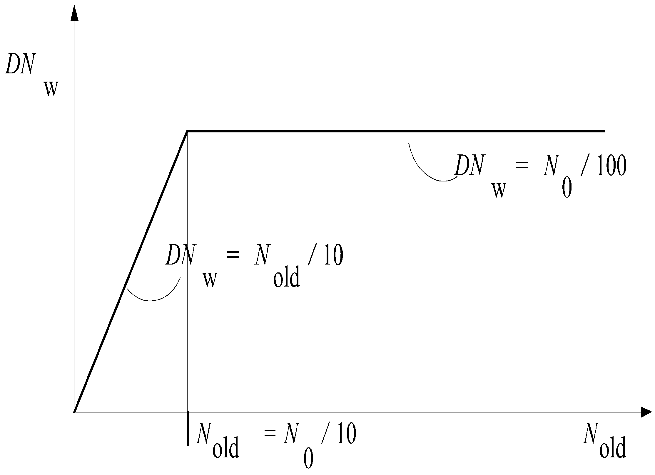
Fig. 4.20.5 DN_w as a function of N

As long as \(N_\text{old} > N_0/10\), DN_w is fixed to DN = \(N_0/100\). At a certain instant the pump speed drops below the value \(N_0/10\). From that moment on DN_w is varying according to DN = \(N_\text{old}/10\). Based on this arbitrarily chosen DN_w a new (sub) time step ∆t^* is calculated in the following way:

• \(N_\text{new}\) is calculated using ∆t (first estimate)

• The difference DN is calculated

• Depending on \(N_\text{old}\), DN_w is calculated (see figure 4)

• The number of (sub) time steps within ∆t is calculated: \(N_\text{t-steps}\) = DN/DN_w

• The new time step ∆t^* = ∆t/\(N_\text{t-steps}\) is calculated.

Once this is done the \(N_\text{new}\) is calculated using ∆t^* (provided that \(N_\text{t-steps}\) > 1) until t = t_old ­+ ∆t.

4.20.1.5. Motor drive

For the motor driven pump the following considerations are to be taken into account. The pump speed is computed using equation (16) of the mathematical model description in the beginning of this section.

(4.20.22)\[T_{d}-T=I_{p} \frac{d N}{d t} \frac{2 \pi}{60}\]

Here, the driving torque \(T_\text{d}\) is determined by the motor properties. In general, when the motor is powered on, \(T_\text{d}\) is a function of the pump speed and the frequency of the speed control. In case the power is off, \(T_\text{d}\) is of course zero and we then have a situation equivalent to the tripping pump.

Typical speed-torque curves for electric motors and diesel engines are plotted below.

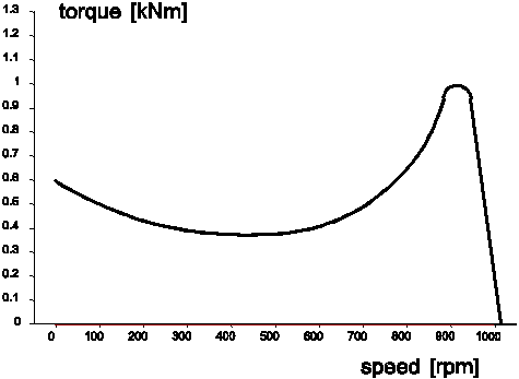
Fig. 4.20.6 Electric motor

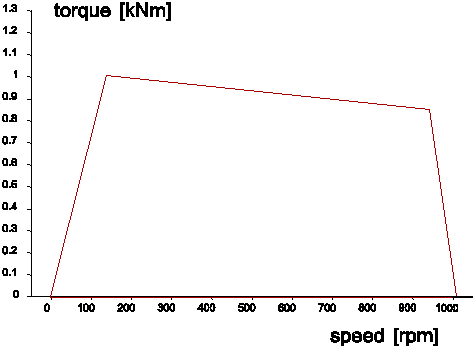
Fig. 4.20.7 Diesel engine

Both curves are characterised by a sharp drop (cut-off) around the operating speed. The result of this is that with load increase the speed does not drop much. This is denoted as elastic behaviour. If the maximum torque just before the drop is sufficiently large the steady state value of the pump speed is well defined. In steady state wanda will compute two equilibria: 1) pump (QH) curve versus system resistance (QH relation) and 2) hydraulic torque versus motor torque. Both are varying at each iteration step and to reach convergence a dedicated iteration strategy has been employed.

For electric motors the pump speed at which the torque goes through zero is denoted by the term “synchronous speed”. This speed is in general equal to 3000 RPM (the frequency of the AC power) divided by the number of coils, which is half the number of poles. In practice many two-coil (four pole) and three-coil (six pole) motors are used with their respective synchronous speeds of 1500 RPM and 1000 RPM. An electric motor can only generate torque if the shaft RPM exhibits a certain “slip” relative to the synchronous speed. The nominal power (and torque) will be delivered at somewhere between 1 and 3 % slip, this is specified by the manufacturer. The peak torque is about 3 times as large as the nominal torque. The start torque is about 2.2 times as large as the nominal torque and the sag torque (the relative minimum half way) is about 2 times the nominal torque.

To be able to “brake” or “force down” the pump by means of a temporarily negative torque, the speed torque table has to be mirrored about the synchronous point. This can easily be done by hand by adding the difference of the synchronous speed and the speed value to the synchronous speed and reversing the torque value of each speed-torque co-ordinate pair. An example is given in figure 7 below:

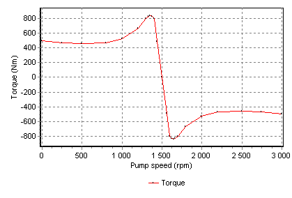
Fig. 4.20.8 Complete speed-torque curve for electric motor

The nominal power for the speed torque curve in figure 7 can be computed by multiplying the nominal torque (which could be 220 Nm) and the speed (which is in that case 155 rad/s). The resulting nominal power is 34.1 kW. However in this case the motor can also run at 150.8 rad/s (1440 RPM) delivering a torque of 490.7 Nm (this is the penultimate co-ordinate just before the synchronous point), leading to a power of 74 kW. The motor slip is in that case 60 RPM. Whether this will lead to thermal problems depends on the design of the motor and this mode of operation has to be confirmed by the manufacturer.

The speed values in the curve are offset by the relative frequency, thus moving the curve in horizontal direction, thereby moving also the synchronous point to the left or right (decreasing or increasing of RPM). Theoretically the relative frequency can even become zero but then the motor torque will be zero throughout. In order to “force” the pump down in RPM the speed-torque curve must also contain negative torque values for speeds greater than the synchronous speed.

In unsteady state the relative frequency should not be changed faster than the pump RPM can follow, otherwise the operating point (intersection between impeller speed-torque and motor speed-torque curves) will drop in the start-up zone.

4.20.2. Pump properties

4.20.2.1. Hydraulic specifications

Description	input	unit	Range	default	remarks
Characteristic type	QHE / Suter			QHE
QHE table	table				if Char. type = QHE
Suter table	table				if Char. type = Suter
Rated speed	real	[rad/s]	(0-1010)
Q in best point of eff.					if Char. type = Suter
H in best point of eff.					if Char. type = Suter
T in best point of eff.					if Char. type = Suter
Initial setting	Speed / H_upstream / H_downstream / Discharge / Frequency			Speed
Initial speed		[rad/s]			if Initial setting = Speed
Initial suction head		[m]			if Initial setting = H_upstream
Initial pressure head		[m]			if Initial setting = H_downstream
Initial discharge		[m3/s]			if Initial setting = Discharge
Initial relative frequency		[-]			if Initial setting = Frequency
Speed-Torque char.of motor	table				if Initial setting = Frequency
Polar moment of inertia	real	[kgm2]	(0-2000]		only in transient mode
Drive type	Steady / Trip / Speed / Motorfreq / Level OnOff / Discharge			Steady
Trip time		[s]			if Drive type = Trip
Action table speed	time vs. speed				if Drive type = Speed
Minimum speed for tripping		[rad/s]			if Drive type = Speed
Action table motorfreq	time vs. rel. motorfreq.				if Drive type = Motorfreq
Minimum rel.freq. for trip.		[-]			if Drive type = Motorfreq
Level On		[m]			if Drive type = Level OnOff
Level Off		[m]			if Drive type = Level OnOff
Start time (0 to max)		[s]			if Drive type = Level OnOff
Stop time (max to 0)		[s]			if Drive type = Level OnOff
Action table discharge	time vs. discharge				if Drive type = Discharge
Required speed	real	[rad/s]	(0-1010)		only visible in system characteristics
Minimum speed	real	[rad/s]	(0-1010)		only visible in pump energy
Maximum speed	Real	[rad/s]	(0-1010)		only visible in pump energy
Maximum power	Real	[W]	(0-1010)		only visible in pump energy

Because the Suter curves are dimensionless the discharge (Q), head (H) and torque (T) in the best efficiency point must also be supplied if the characteristic type is “Suter”.

In case of the QHE characteristic the Q and H at maximum efficiency will be found in the table. Hence the user must take care for one maximum value within the E range.

Used table types

QHE table (Q to run from 0.0 upwards, H to decrease monotonously, E to be zero at either H=0.0 or Q=0.0)

Q	H	E
[m3/s]	[m]	[-]
Real	Real	Real
…	…	…
…	…	…
real	real	real

Suter table (x/π to run from 0.0 to 2.0)

x/π	WH	WB
[-]	[-]	[-]
Real	Real	Real
…	…	…
…	…	…
real	real	real

Three Suter curves according to Wylie and 14 curves according to Thorley have been included as property templates (see …Wanda3Property templatesExamplesSuter_pump)

Speed torque table in case of motor driven pump (see examples)

N	T
[rad/s]	[Nm]
Real	Real
…	…
…	…
real	real

Important:

• Minimum required rows is 5, maximum is 100.

• The heads in the Q-H table must be monotonously decreasing.

• The Q-E table must have a maximum value for the efficiency E.

• Efficiency must be zero where either Q=0 or H=0.

• It is recommended to start QHE tables with Q = 0 [m³/s].

• The first and last row values of WH and WB should respectively have the same values (for x/π=0 and x/π=2), thus forming closed curves.

Steady state settings

To determine the steady state condition of the pump the choice property “Initial setting” has to be set accordingly. The user has five choices:

Speed	The operational speed is specified by the user. QH curve will be applied in computation and H1, H2 and Q are computed depending on system
H_upstream	The head upstream is specified by the user. H1 = C is applied in computation and H2 and Q are computed. Afterwards, the pump speed will be computed, such that the combination H2-H1 and Q is on the QH curve.
H_downstream	The head downstream is specified by the user. H2 = C is applied in computation and H2 and Q are computed. Afterwards, the pump speed will be computed, such that the combination H2-H1 and Q is on the QH curve.
Discharge	The discharge is specified by the user. Q = C is applied in computation and H2 and Q are computed. Afterwards, the pump speed will be computed, such that the combination H2-H1 and Q is on the QH curve.
Frequency	The relative motor frequency is specified by the user. This is the actual frequency (e.g. 40 Hz) divided by the nominal frequency (e.g. 50 Hz) yielding the value of 0.8. With this relative frequency the speed-torque curve of the motor is adapted (shifted horizontally) and the steady state (H1, H2 and Q) will be solved such that motor torque and hydraulic (impeller) torque intersect. The point of intersection determines the actual pump speed.

Unsteady state settings

For the computation of the pump during unsteady state there are five possibilities to choose from in the property “Drive type”

Steady	The pump speed and the QH curve will be kept constant, throughout the complete simulation time. Value for “polar moment of inertia” is not used
Trip	The pump speed and QH curve will be maintained until the user specified “trip time”. Thereafter the motor torque will be zero and the pump will trip according to equation 15.
Speed	The pump speed will be determined by applying the time-speed table (which is specified by the user). Polar moment of inertia is not taken into account during use of the table If the value in the field”min speed for tripping” has been undershoot, the speed table is overruled and the pump acts as a tripping pump, see remark 3
Motorfreq	The pump speed will be computed by applying the transformed speed-torque curve of the motor on basis of the time table for the relative frequency (which is specified by the user)
Level OnOff	Fixed speed pump is switched on if upstream head H1 > “Level On”; speed increases in “Start time” seconds from 0 to “Rated speed” Pump is switched off if upstream head H1 < “Level Off”; speed decreases in “Stop time” seconds from rated speed to 0 Polar moment of inertia is not taken into account This pump type can be used for simple pump operation control; use Control module for advanced operational control
Discharge	This pump drive type is used to prescribe the discharge over time by means of an action table or a signal line from a control loop. The pump speed will be computed

Remarks

• It is most logical to apply drive type “Speed” in combination with initial setting “Speed” and drive type “Motorfreq” in combination with initial setting “Frequency” in order to have a smooth transition between the steady state and unsteady state computations. However, different combinations are in principle possible. The user must take care that the pump speeds match between steady and unsteady. Differences will however be solved dynamically: the unsteady state solution process aims at achieving a new balance.

• All “Drive type” types may be controlled by a control loop (C-components).

• To trigger the “trip” action on a pump with drivetype = speed at certain point in time T, the table value of the speed before T must be greater than the value of the input property “Minimum speed for tripping” and the table value after T must be equal to zero.

4.20.2.2. Component messages

Message	Type	Explanation
Q‑H curve not monotonously Decreasing	Warning	To prevent instability, the derivative of H(Q) must be negative.
Pump efficiency must be zero if either Q=0 or H=0 in input and non‑zero elsewhere	Error	To have a finite torque, this is by definition.
Pump specific speed =…	Info	Small number (<40) denotes centrifugal pump, large num­ber (>100) denotes axial pump.
Pump efficiency less than 0 or greater than 1	Error
Motor overloaded Fluid torque = … [kNm] Max. motor torque = … [kNm]	Error	The intersection between hydraulic and motor torque is at the left of the maximum motor torque.
Convergence between fluid and motor torque less accurate than 0.1 % Fluid torque = … [kNm] Motor torque = … [kNm]	Warning	This will lead to a further conver­gence process in transient, therefore we are not yet in a steady state.
Initial pump speed = … [rpm]	Info	.
Initial‑running status contradictive with control based running status	Warning	For example, according to the initial status the suction controlled pump is running, whereas the measured suc­tion level is below the switch off level.
Unbalance exceeding rpm sensitivity fluid torque = … Nm motor torque = … Nm	Warning	Within the accuracy of pump speed computation, it was not possible to obtain balance between hydraulic and motor torques. The pump speed is correct however and the torque unbal­ance will settle during the following time steps (dynamics).
Starts	Info	.
Initial value of action table does not coincide with initial value of pump speed.	Warning	A possibly unintended “jump” in the pump speed will occur upon starting the unsteady state computation.
Motor overloaded	Warning	The hydraulic torque has become larger than the maximum (peak) motor torque. The motor is not longer capable of holding the normal pump speed. This is called a powered trip.
Trips	Info	.
Inconsistent pump speed between steady state results and control system; steady state value will be used	Warning	Message given if discrepancy between steady state speed and control value is less than 1 %
Inconsistent pump speed between steady state results and control system; Modify input	Error	Message given if discrepancy between steady state speed and control value is more than 1 %

4.20.2.3. Component specific output

Pump speed [rad/s]

Fluid torque [Nm]

Motor torque [Nm]

On/Off [-]

Efficiency [-]

Power [W].

4.20.2.4. H-actions

How to activate the pump is dependent of the drive type. If the type is “steady” there will be no action applicable. The pump just keeps running and the fixed QH-curve will apply throughout the steady state computation. The speed may be overruled by a control connection (signal line).

If the drive type is “trip” the input value “trip time” will determine the time at which the driving torque becomes zero and the pump speed will solely be determined by the hydraulic torque. The speed may be overruled by a control connection (signal line)

If the drive type is “speed” the applicable action table will be of the time-speed type. In case the initial control is also “speed” the user interface will copy the initial speed into the table. In other cases (init_H1, init_H2, init_Q and motor), the initial pump speed will be calculated by the computational core (STEADY) and it is the user’s responsibility to have the time-speed table starting with the same pump speed. A warning will be issued however in case of a discrepancy. The action table may be overruled by a control connection (signal line).

If the drive type is “MotorFreq” the action table will be of the type “relative frequency” which is in effect a dimensionless table. The percentage will be used to scale the motor speed-torque curve relative to the y-axis (speeds will be multiplied with the scaling factor). The action table may be overruled by a control connection (signal line).

If the drive type is “Level On/Off” the pump acts as a start/stop pump if the upstream head over/undershoot the On/Off values specified. The speed increase/decrease is defined by the ramp parameters.

If the drive type is “Discharge” then the pump will follow a time dependent discharge program, either specified in an action tabel, or specified by means of a signal line from a control loop.