4.10. Control valve

4.10.1. FCV

Fig. 4.10.1 Flow control valve

Fall type

type label	description	active
Flow control valve	Flow control valve (FCV).	yes

4.10.1.1. Mathematical model

This valve controls the flow rate by adjusting the valve position. The basic pressure loss equation for a Newtonian fluid and without cavitation is:

(4.10.1)\[\Delta H=\xi(\theta) \frac{v^{2}}{2 g}\]

(4.10.2)\[H=z+\frac{p}{\rho g}\]

in which:

Variable	Description	Units
∆H	pressure head difference across the valve	m
\(\xi\)	valve position dependent loss coefficient	-
\(\theta\)	valve position	-
g	gravitational acceleration	m/s2
v	velocity	m/s
z	elevation	m
p	pressure	N/m2
ρ	density of the fluid	kg/m3

Note that z₁ (upstream) and z₂ (downstream) are not necessarily the same, so the sign of the pressure difference may be even opposite to the head difference with the same flow.

Instead of the loss characteristic, the discharge coefficients K_v or C_v may also be used:

(4.10.3)\[K_{v}=\frac{Q}{\sqrt{\Delta p}}\]

with:

Variable	Description	Units
Kv	discharge coefficient	m3/h/√bar
Q	flow	m3/h
\(\Delta p\)	net pressure difference across the valve	bar

In words: the discharge coefficient K_v denotes the water flow rate in m³/h through a valve at a pressure difference of 1 bar.

Apart from K_v, C_v is also defined as a discharge coefficient for American units.

(4.10.4)\[C_{v}=\frac{Q}{\sqrt{\Delta p}}\]

with

Variable	Description	Units
Cv	discharge coefficient	USGPM/√psi
Q	flow	US gallons/min
\(\Delta p\)	Net pressure difference across the valve	psi

The relation between ξ, Kv and Cv is as follows:

(4.10.5)\[\xi=1.6 \cdot 10^{9} \frac{1}{K_{v}^{2}} D^{4}\]

(4.10.6)\[K_{v}=0.865 C_{v}\]

A valve is characterised by = f ( ) or K_v = f ( ) or C_v = f ( ).

denotes the dimensionless valve opening. ranges from 0 to 1 (in SI-units, or 0 to 100% in percentage annotation).

= 0, valve is closed (0% open)

= 1, valve is completely open (100% open).

The different discharge characteristics are always translated to the following equation:

(4.10.7)\[\Delta H=a \xi Q_{1}\left|Q_{1}\right|\]

in which:

Variable	Description	Units
∆H	H1 ‑ H2 in positive flow direction	m
H1	upstream head	m
H2	downstream head	m
a	1 / (2 g Af2)	s2/m5
\(\xi\)	loss coefficient	‑
Q1	discharge upstream	m3/s
Af	discharge area valve	m2

The discharge characteristic may be defined by one of Deltares’ standard characteristics (See Hydraulic specifications) or by a user-defined discharge characteristic. If the valve position does not coincide with a tabulated position, interpolation must be performed to obtain the discharge coefficient for intermediate valve positions. The standard characteristics and the user-defined ξ characteristic are interpolated logarithmically according to the following equation:

(4.10.8)\[\begin{split}\begin{array}{l} \theta(z)=z \cdot \theta_{1}+(1-z) \cdot \theta_{2} \\ \xi(\theta(z))=\xi_{1}^{z} \cdot \xi_{2}^{1-z} \end{array}\end{split}\]

The user-defined K_v and C_v characteristics are interpolated such that K_v or C_v values are interpolated linearly:

(4.10.9)\[\frac{1}{\sqrt{\xi(\theta(z))}}=\frac{z}{\sqrt{\xi_{1}}}+\frac{1-z}{\sqrt{\xi_{2}}}\]

in which:

Variable	Description	Units
\(\theta_{1}, \theta_{2}\)	tabulated valve positions	-
\(\xi\)	fraction, which defines intermediate valve position (0 < z < 1)	-
\(\theta(\xi)\) )	intermediate valve position	-
\(\xi_{1}, \xi_{2}\) 2	loss coefficient at \(\theta_{1}, \theta_{2}\)	‑
\(\xi(\theta(z))\)	interpolated loss coefficient	‑

If the valve is fully closed the governing equation is:

(4.10.10)\[Q_{1}=0\]

Controlling actions

This valve controls the flow rate by adjusting the valve position. The valve position is adjusted with a speed proportional to the error (measured value minus set value: error = Q₁ – Q_set). The speed is truncated to the full stroke closing speed if the absolute value of the error is greater than the proportionality range.

(4.10.11)\[\dot{\theta}_{\text {valve }}=\frac{Q_{1}-Q_{\text {set }}}{Q_{\text {cutoff }} T_{\mathrm{c}}} \quad \wedge \quad \text { abs }\left(\dot{\theta}_{\text {valve }}\right) \leq \frac{1}{T_{\mathrm{c}}}\]

in which:

Variable	Description	Units
\(\dot{\theta}_{\text {valve }}\)	(angular) velocity of valve	s-1
Q1	discharge	m3/s
Qset	set discharge	m3/s
Qcutoff	proportionality range	m3/s
Tc	full stroke closing time	s

For the initial situation either the valve position or the flow rate can be prescribed. In case the initial position is prescribed, the computed flow rate will generally differ from the set value. The set value will then be attained during the unsteady state computation. In case the initial flow rate is chosen to be the set value, the valve position will be determined on basis of the hydraulic solution. This is the preferred method if a balanced start of the unsteady state computation is required.

The maximum and minimum valve position may be different from 1 (100 % open) and 0 (fully closed) respectively by defining the valve characteristic table only between the desired lower and the upper limits. For example if the characteristic is specified as:

position θ	loss coef. ξ
0.3	5600
0.4	1600
0.5	900
0.6	500
0.7	300

The valve position will remain within 0.3 and 0.7. The initial position must also be within these limits or an error message will result. This is not applicable for the standard valve characteristics.

The controlling action is defined in the table below. The normal action is with a positive head difference and flow (hence: H₁ > H₂). This is shown in the second column of the table. For a negative head difference the valve will go to the minimum valve position (normally fully closed), since the (always positive) set value can not be reached. This is shown in the third column.

Q ctrl (FCV)	H1 > H2	H1 < H2
Q < Qset		\(\downarrow\)
Q > Qset		\(\downarrow\)

In which:

: open further until set value reached;

: close further until set value reached;

\(\downarrow\): go to the minimum valve position (normally fully closed) at maximum speed;

Cavitation

Cavitation depends on the pressure conditions around the valve. Usually these pressure conditions are defined by a pressure relation. Several different definitions are use in the industrial standards.

In WANDA the factor Xf is used, according the German VDMA standard.

(4.10.12)\[X_{f}=\frac{\Delta p}{p_{1}-p_{v}}\]

in which:

Variable	Description	Units
Xf	pressure ratio	-
∆p	net pressure difference across the valve	N/m2
p1	absolute pressure upstream of the valve	N/m2
pv	vapour pressure of the fluid	N/m2

The pressure ratio depends of the valve opening: X_f = f (θ)

The pressure ratio X_f is only calculated for positive flow; for negative flow X_f = 0.

If the cavitation characteristic is specified, the program calculates the pressure ratio in the system and warns the user if it exceeds the available value as defined in the characteristic.

Note:

In other standards (ISA, BS, IEC) the pressure ratio \(X_{T}\) is used:

(4.10.13)\[X_{T}=\frac{p_{1}-p_{2}}{p_{1}}=\frac{\Delta p}{p_{1}}\]

In some standards (e.g. ISA) the Thoma number σ is used. \(\sigma=\frac{p_{1}-p_{v}}{\Delta p}\)

in which:

Variable	Description	Units
σ	pressure ratio	-
∆p	net pressure difference across the valve	N/m2
P1	absolute pressure upstream of the valve	N/m2
pv	vapour pressure of the fluid	N/m2

The relationship between Xf and σ is: \(\sigma=\frac{1}{X_{f}}\)

Another definition for the Thoma number is based on the downstream pressure p2:

(4.10.14)\[\sigma_{2}=\frac{p_{2}-p_{v}}{\Delta p}\]

where \(\sigma=1+\sigma_{2}\) and \(\sigma_{2}=\frac{1}{X f}-1\)

Remarks

None

4.10.1.2. Hydraulic specifications

Description	input	Unit	range	default	remarks
Characteristic type	Standard/ Kv/ Cv/ Xi
Standard type	Buttrfly/ Ball/ Gate/ Gate_sqr			Buttrfly	if char.type = Standard
Kv characteristic	Table				if char.type = Kv
Cv characteristic	Table				if char.type = Cv
Xi characteristic	Table				if char.type = Xi
Inner diameter	Real	[m]	(0-1000]
Initial setpoint	Real	[m3/s]	(0-10]		does not have to be the same as the initial flow
Initial setting	Position / Discharge
Initial position (open)	Real	[-]	[0-1]		0 = closed 1 = open If init_setting = Position
Initial discharge	Real	[m3/s]	(0, 10]		If init_setting = Discharge
Full stroke closing time	Real	[s]	(0-107]
Proportionality range	Real	[m3/s]			Related to error see mathematical model
Check cavitation	Yes/No
Cavitation table	Table				If check cavitation = Yes

4.10.1.3. Component specific output

Valve position [-]

Pressure ratio X_f system [-]

4.10.1.4. H-actions

The setpoint of the valve can be changed over time by means of the action table.

Example action table:

Time [s]	Discharge [m3/s]
0	1.0
10	1.0
20	2.0

Note:

The setpoint may be also changed by a control signal line; the control signal line overrules the action table.

4.10.1.5. Component messages

Message	Type	Explanation
Valve resistance in max. open position too large to obtain prescribed state or Valve resistance in min. open position too small to obtain prescribed state	Info	The specified discharge cannot be obtained. The required loss coefficient is outside of the bounds of the valve characteristic. Either increase valve table or adjust settings.
Initial setting not physically realistic Discharge opposite to pressure drop	Info	The specified discharge cannot be obtained. Change initial discharge value or change setting to position
Inconsistent valve position between steady state results and action table	Info	If difference is less than 1% value of action table will be used otherwise user had to change input
Start controlling	Info	The valve (re)opens and starts balancing
Closes	Info	Valve fully closed; position is 0
Reaching maximum opening	Info	Valve runs out of control; capacity in maximum open position to small too obtain required upstream pressure
Reaching minimum opening	Info	Valve runs out of control; capacity in minimum open position to large too obtain required upstream pressure

4.10.1.6. Example

A flow control valve is located in the middle of a 1000 m long pipeline.

The initial position of the valve is set to 40 % open. The steady state discharge is 140 m³/h bar. The required discharge is 200 m³/h.

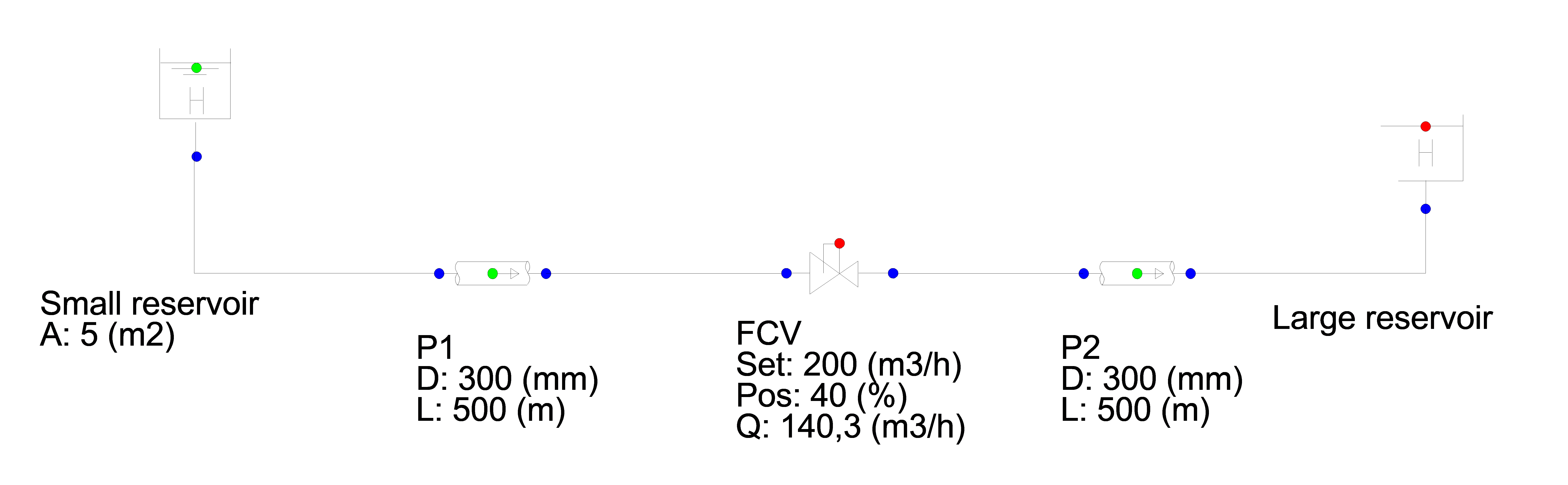
Fig. 4.10.2 Schematic Wanda model

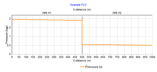
Fig. 4.10.3 Pressure over x-distance along both pipe 1 and pipe 2

In the unsteady state the FCV starts controlling. Due to the decreasing level in the small reservoir the PdCV adjusts the position continuously to maintain the set discharge (200 m³/h).

At t= 500 sec, the setpoint has been changed to 100 m³/h(via the action table).

Next figure shows the results.

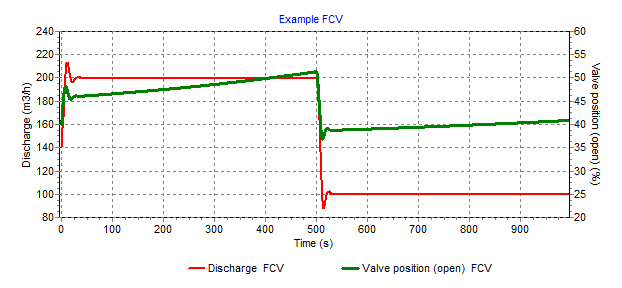
Fig. 4.10.4 Discharge through the flow control valve (FCV) and opening position of the FCV over time.

4.10.2. PdCV

Fig. 4.10.5 Downstream pressure control valve

Fall type

type label	description	active
Downstream pressure control valve	Also known as pressure reducing valve (PRV).	yes

4.10.2.1. Mathematical model

This valve controls the pressure downstream by adjusting the valve position. The basic pressure loss equation for a Newtonian fluid and without cavitation is:

(4.10.15)\[\Delta H=\xi(\theta) \frac{v^{2}}{2 g}\]

(4.10.16)\[H=z+\frac{p}{\rho g}\]

in which:

Variable	Description	Units
∆H	pressure head difference across the valve	m
\(\xi\)	valve position dependent loss coefficient	-
\(\theta\)	valve position	-
g	gravitational acceleration	m/s2
v	velocity	m/s
z	elevation	m
p	pressure	N/m2
ρ	density of the fluid	kg/m3

Note that z₁ (upstream) and z₂ (downstream) are not necessarily the same so the sign of the pressure difference may be even opposite to the head difference with the same flow.

Instead of the loss characteristic, the discharge coefficients K_v or C_v may also be used:

(4.10.17)\[K_{v}=\frac{Q}{\sqrt{\Delta p}}\]

with:

Variable	Description	Units
Kv	discharge coefficient	m3/h/√bar
Q	flow	m3/h
∆p	net pressure difference across the valve	bar

In words: the discharge coefficient K_v denotes the water flow rate in m³/h through a valve at a pressure difference of 1 bar.

Besides K_v, C_v is also defined as a discharge coefficient for American units.

(4.10.18)\[C_{v}=\frac{Q}{\sqrt{\Delta p}}\]

with

Variable	Description	Units
Cv	discharge coefficient	USGPM/√psi
Q	flow	US gallons/min
∆p	Net pressure difference across the valve	psi

The relation between ξ, Kv and Cv is as follows:

(4.10.19)\[\xi=1.6 \cdot 10^{9} \frac{1}{K_{v}^{2}} \cdot D^{4}\]

(4.10.20)\[K_{v}=0.865 C_{v}\]

A valve is characterised by ξ = f (θ ) or K_v = f (θ ) or C_v = f (θ ).

θ denotes the dimensionless valve opening. θ ranges from 0 to 1 (in SI-units, or 0 to 100% in percentage annotation).

• = 0, valve is closed (0% open)

• = 1, valve is completely open (100% open)

The different discharge characteristics are always translated to the following equation:

(4.10.21)\[\Delta H=a \xi Q_{1}\left|Q_{1}\right|\]

in which:

Variable	Description	Units
∆H	H1 ‑ H2 in positive flow direction	m
H1	upstream head	m
H2	downstream head	m
a	1 / (2 g Af2)	s2/m5
\(\xi\)	loss coefficient	‑
Q1	discharge upstream	m3/s
Af	discharge area valve	m2

The discharge characteristic may be defined by one of Deltares’ standard characteristics (See Hydraulic specifications) or by a user-defined discharge characteristic. If the valve position does not coincide with a tabulated position, interpolation must be performed to obtain the discharge coefficient for intermediate valve positions. The standard characteristics and the user-defined ξ characteristic are interpolated logarithmically according to the following equation:

(4.10.22)\[\begin{split}\begin{array}{l} \theta(z)=z \cdot \theta_{1}+(1-z) \cdot \theta_{2} \\ \xi(\theta(z))=\xi_{1}^{z} \cdot \xi_{2}^{1-z} \end{array}\end{split}\]

The user-defined K_v and C_v characteristics are interpolated such that K_v or C_v values are interpolated linearly:

(4.10.23)\[\frac{1}{\sqrt{\xi(\theta(z))}}=\frac{z}{\sqrt{\xi_{1}}}+\frac{1-z}{\sqrt{\xi_{2}}}\]

in which:

Variable	Description	Units
\(\theta_{1,}, \theta_{2}\)	tabulated valve positions	-
\(\xi\)	fraction, which defines intermediate valve position (0 < z < 1)	-
\(\theta(\xi)\)	intermediate valve position	-
\(\xi_{1}, \xi_{2}\) 2	loss coefficient at \(\theta_{1}, \theta_{2}\)	-
\(\xi(\theta(z))\)	interpolated loss coefficient	-

If the valve is fully closed the governing equation is:

(4.10.24)\[Q_{1}=0\]

Controlling actions

This valve controls the pressure downstream by adjusting the valve position. The valve position is adjusted with a speed proportional to the error (measured value minus set value: error = p₂ – p_set). The speed is truncated to the full stroke closing speed if the absolute value of the error is greater than the proportionality range.

(4.10.25)\[\dot{\theta}_{\text {valve }}=\frac{p_{2}-p_{\text {set }}}{p_{\text {cutoff }} T_{\mathrm{c}}} \quad \wedge \quad \operatorname{abs}\left(\dot{\theta}_{\text {valve }}\right) \leq \frac{1}{T_{\mathrm{c}}}\]

in which:

Variable	Description	Units
\(\dot{\theta}_{\text {valve }}\)	(angular) velocity of valve	s-1
p2	downstream pressure	N/m2
pset	set pressure	N/m2
pcutoff	proportionality range	N/m2
Tc	full stroke closing time	s

For the initial situation either the valve position or the set value can be chosen. In case the initial position is prescribed, the computed pressure will generally differ from the set value. The set value will then be attained during the unsteady state computation. In case the initial setting is chosen to be the set value, the valve position will be determined on basis of the hydraulic solution. This is the preferred method if a balanced start of the unsteady state computation is required.

The maximum and minimum valve position may be different from 1 and 0 respectively by defining the valve characteristic table only between the desired lower and the upper limits. For example if the characteristic is specified as:

position θ	loss coef. ξ
0.3	5600
0.4	1600
0.5	900
0.6	500
0.7	300

The valve position will remain between 0.3 and 0.7. The initial position must also be within this range or an error message will result. This is not applicable for the standard valve characteristics.

The controlling action is defined in the table below. The normal action is with a positive head difference and flow (hence: H₁ > H₂). This is shown in the second column of the table. H_set is the set pressure head at the downstream node. In the third column the action is shown if the set value can not be reached but the error is minimised. This will lead to fully opening.

For a negative head difference (that means negative flow) the valve will go to the minimum valve position (normally fully closed). This is shown in the fourth column

p2 ctrl (PRV)	H1 > H2	H1 < H2
	H1 > Hset	H1 < Hset
p2 < pset			\(\downarrow\)
p2 > pset			\(\downarrow\)

In which:

: open further until set value reached;

: open fully, set value will not be reached;

: close further until set value reached;

\(\downarrow\) : go to the minimum valve position (normally fully closed) at maximum speed;

: not applicable

The valve will close if the valve position becomes zero.

The valve will start controlling if there is a positive pressure head difference (H₁ > H₂) and the upstream pressure is above the setpressure (p₁ > p_set).

Cavitation

Cavitation depends on the pressure conditions around the valve. Usually these pressure conditions are defined by a pressure relation. Several different definitions are use in the industrial standards.

In WANDA the factor Xf is used, according the German VDMA standard.

(4.10.26)\[X_{f}=\frac{\Delta p}{p_{1}-p_{v}}\]

in which:

Variable	Description	Units
Xf	pressure ratio	-
∆p	net pressure difference across the valve	N/m2
p1	absolute pressure upstream of the valve	N/m2
pv	vapour pressure of the fluid	N/m2

The pressure ratio depends of the valve opening: X_f = f (θ)

The pressure ratio X_f is only calculated for positive flow; for negative flow X_f = 0.

If the cavitation characteristic is specified, the program calculates the pressure ratio in the system and warns the user if it exceeds the available value as defined in the characteristic.

Note:

In other standards (ISA, BS, IEC) the pressure ratio \(X_{T}\) is used:

(4.10.27)\[X_{T}=\frac{p_{1}-p_{2}}{p_{1}}=\frac{\Delta p}{p_{1}}\]

In some standards (e.g. ISA) the Thoma number σ is used. \(\sigma=\frac{p_{1}-p_{v}}{\Delta p}\)

in which:

Variable	Description	Units
σ	pressure ratio	-
∆p	net pressure difference across the valve	N/m2
P1	absolute pressure upstream of the valve	N/m2
pv	vapour pressure of the fluid	N/m2

The relationship between Xf and σ is: \(\sigma=\frac{1}{X_{f}}\)

Another definition for the Thoma number is based on the downstream pressure p2:

(4.10.28)\[\sigma_{2}=\frac{p_{2}-p_{v}}{\Delta p}\]

where \(\sigma=1+\sigma_{2}\) and \(\sigma_{2}=\frac{1}{X f}-1\)

4.10.2.2. Hydraulic specifications

Description	input	Unit	range	default	remarks
Characteristic type	Standard/ Kv/ Cv/ Xi
Standard type	Buttrfly/ Ball/ Gate/ Gate_sqr			Buttrfly	if char.type = Standard
Kv characteristic	Table				if char.type = Kv
Cv characteristic	Table				if char.type = Cv
Xi characteristic	Table				if char.type = Xi
Inner diameter	Real	[m]	(0-1000]
Initial setpoint	Real	[N/m2]	[-105 – 107]		does not have to be the same as the initial pressure
Initial setting	Position / P_downstr
Initial position (open)	Real	[-]	[0-1]		0 = closed 1 = open If init_setting = Position
Initial downstream pressure	Real	[N/m2]	[-105 – 107]		If init_set = P_downstr
Full stroke closing time	Real	[s]	(0-107]
Proportionality range	Real	[N/m2]			Related to error see mathematical model
Check cavitation	Yes/No
Cavitation table	Table				If check cavitation = Yes

4.10.2.3. Component specific output

Valve position [-]

Pressure ratio X_f system [-]

4.10.2.4. H-actions

The setpoint of the valve can be changed over time by means of the action table.

Table 4.10.1 Example action table

Time [s]	Pressure [N/m2]
0	7⋅105
10	7⋅105
20	5⋅105

Note:

The setpoint may be also changed by a control signal line; the control signal line overrules the action table.

4.10.2.5. Component messages

Message	Type	Explanation
Valve resistance in max. open position too large to obtain prescribed state or Valve resistance in min. open position too small to obtain prescribed state	Info	The specified downstream pressure cannot be obtained. The required loss coefficient is outside of the bounds of the valve characteristic. Either increase valve table or adjust settings.
Initial setting not physically realistic Discharge opposite to pressure drop	Info	The specified downstream pressure cannot be obtained. Change initial downstream pressure value or change setting to position
Inconsistent valve position between steady state results and action table	Info	If difference is less than 1% value of action table will be used otherwise user had to change input
Start controlling	Info	The valve (re)opens and starts balancing
Closes	Info	Valve fully closed; position is 0
Reaching maximum opening	Info	Valve runs out of control; capacity in maximum open position to small too obtain required upstream pressure
Reaching minimum opening	Info	Valve runs out of control; capacity in minimum open position to large too obtain required upstream pressure

4.10.2.6. Example

A pressure control valve is located in the middle of a 1000 m long pipeline.

The initial position of the valve is set to 80 % open. The steady state downstream pressure is 0.914 bar. The required pressure is 0.7 bar.

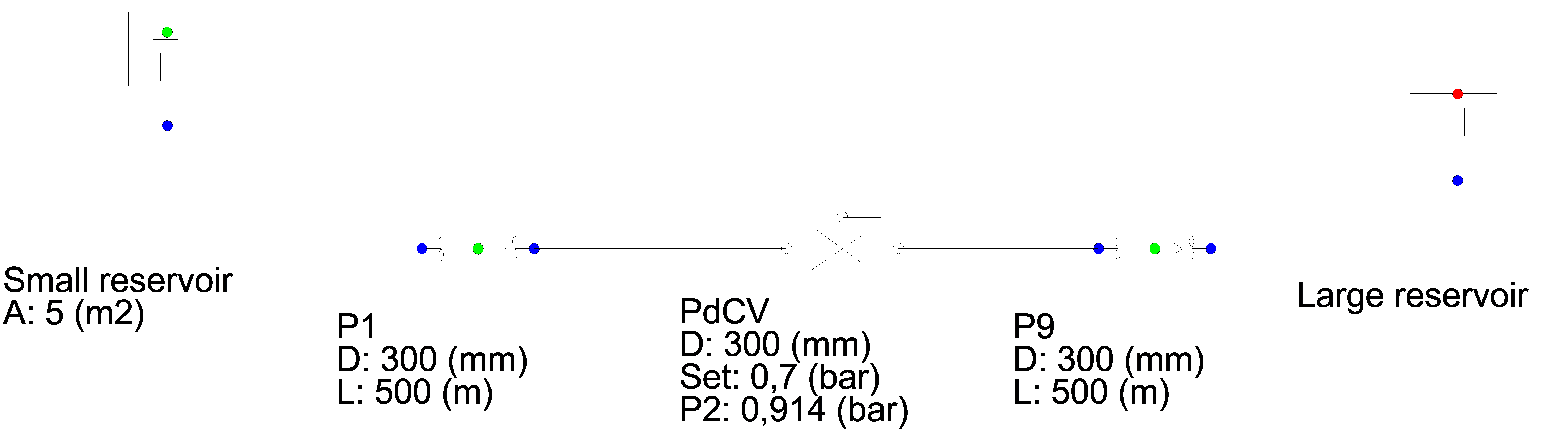
Fig. 4.10.6 Schematic overview of the Wanda model

Fig. 4.10.7 Pressure over x-distance along pipe P1 and P9

In the unsteady state the PdCV starts controlling. Due to the decreasing pressure in the small reservoir the PdCV adjusts the position continuously to maintain the set pressure (0.7 bar).

At T= 300 sec, the setpressure has been changed to 0.5 bar (via the action table).

Next figure shows the results.

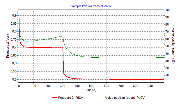
Fig. 4.10.8 Pressure and valve position over time for Pressure control valve (PdCV)

4.10.3. PuCV

Fig. 4.10.9 Upstream pressure control valve

Fall type

type label	description	active
Upstream pressure control valve	Also known as pressure sustaining valve (PSV).	yes

4.10.3.1. Mathematical model

This valve controls the pressure upstream by adjusting the valve position. The basic pressure loss equation for a Newtonian fluid and without cavitation is:

(4.10.29)\[\Delta H=\xi(\theta) \frac{v^{2}}{2 g}\]

(4.10.30)\[H=z+\frac{p}{\rho g}\]

in which:

Variable	Description	Units
∆H	pressure head difference across the valve	m
\(\xi\)	valve position dependent loss coefficient	-
\(\theta\)	valve position	-
g	gravitational acceleration	m/s2
v	velocity	m/s
z	elevation	m
p	pressure	N/m2
ρ	density of the fluid	kg/m3

Note that z₁ (upstream) and z₂ (downstream) are not necessarily the same so the sign of the pressure difference may be even opposite to the head difference with the same flow.

Instead of the loss characteristic, the discharge coefficients K_v or C_v may also be used:

(4.10.31)\[K_{v}=\frac{Q}{\sqrt{\Delta p}}\]

with:

Variable	Description	Units
Kv	discharge coefficient	m3/h/√bar
Q	flow	m3/h
∆p	net pressure difference across the valve	bar

In words: the discharge coefficient K_v denotes the water flow rate in m³/h through a valve at a pressure difference of 1 bar.

Besides K_v, C_v is also defined as a discharge coefficient for American units.

(4.10.32)\[C_{v}=\frac{Q}{\sqrt{\Delta p}}\]

with

Variable	Description	Units
Cv	discharge coefficient	USGPM/√psi
Q	flow	US gallons/min
∆p	Net pressure difference across the valve	psi

The relation between ξ, Kv and Cv is as follows:

(4.10.33)\[\xi=1.6 \cdot 10^{9} \frac{1}{K_{v}^{2}} \cdot D^{4}\]

(4.10.34)\[K_{v}=0.865 C_{v}\]

A valve is characterised by ξ = f (θ ) or K_v = f (θ ) or C_v = f (θ ).

θ denotes the dimensionless valve opening. θ ranges from 0 to 1 (in SI-units, or 0 to 100% in percentage annotation).

= 0, valve is closed (0% open)

= 1, valve is completely open (100% open)

The different discharge characteristics are always translated to the following equation:

(4.10.35)\[\Delta H=a \xi Q_{1}\left|Q_{1}\right|\]

in which:

Variable	Description	Units
∆H	H1 ‑ H2 in positive flow direction	m
H1	upstream head	m
H2	downstream head	m
a	1 / (2 g Af2)	s2/m5
\(\xi\)	loss coefficient	‑
Q1	discharge upstream	m3/s
Af	discharge area valve	m2

The discharge characteristic may be defined by one of Deltares’ standard characteristics (See Hydraulic specifications) or by a user-defined discharge characteristic. If the valve position does not coincide with a tabulated position, interpolation must be performed to obtain the discharge coefficient for intermediate valve positions. The standard characteristics and the user-defined ξ characteristic are interpolated logarithmically according to the following equation:

(4.10.36)\[\begin{split}\begin{array}{l} \theta(z)=z \cdot \theta_{1}+(1-z) \cdot \theta_{2} \\ \xi(\theta(z))=\xi_{1}^{z} \cdot \xi_{2}^{1-z} \end{array}\end{split}\]

The user-defined K_v and C_v characteristics are interpolated such that K_v or C_v values are interpolated linearly:

(4.10.37)\[\frac{1}{\sqrt{\xi(\theta(z))}}=\frac{z}{\sqrt{\xi_{1}}}+\frac{1-z}{\sqrt{\xi_{2}}}\]

in which:

Variable	Description	Units
\(\theta_{1}, \theta_{2}\)	tabulated valve positions	-
\(\xi\)	fraction, which defines intermediate valve position (0 < z < 1)	-
\(\theta(\xi)\) )	intermediate valve position	-
\(\xi_{1}, \xi_{2}\) 2	loss coefficient at \(\theta_{1}, \theta_{2}\)	-
(4.10.38)\[\xi(\theta(z))\]	interpolated loss coefficient	-

If the valve is fully closed the governing equation is:

(4.10.39)\[Q_{1}=0\]

Controlling actions

This valve controls the pressure upstream by adjusting the valve position. The valve position is adjusted with a speed proportional to the error (measured value minus set value: error = p₁ – p_set). The speed is truncated to the full stroke closing speed if the absolute value of the error is greater than the proportionality range.

(4.10.40)\[\dot{\theta}_{\text {valve }}=\frac{p_{1}-p_{\text {set }}}{p_{\text {range }} T_{\mathrm{c}}} \quad \wedge \quad \text { abs }\left(\dot{\theta}_{\text {valve }}\right) \leq \frac{1}{T_{\mathrm{c}}}\]

in which:

Variable	Description	Units
\(\dot{\theta}_{\text {valve }}\)	(angular) velocity of valve	s-1
p1	upstream pressure	N/m2
pset	set pressure	N/m2
prange	proportionality range	N/m2
Tc	full stroke closing time	s

For the initial situation either the valve position or the set value can be chosen. In case the initial position is prescribed, the computed pressure will generally differ from the set value. The set value will then be attained during the unsteady state computation. In case the initial setting is chosen to be the set value, the valve position will be determined on basis of the hydraulic solution. This is the preferred method if a balanced start of the unsteady state computation is required.

The maximum and minimum valve position may be different from 1 (100 % open) and 0 (fully closed) respectively by defining the valve characteristic table only between the desired lower and the upper limits. For example if the characteristic is specified as:

position θ	loss coef. ξ
0.3	5600
0.4	1600
0.5	900
0.6	500
0.7	300

The valve position will remain between 0.3 and 0.7. The initial position must also be within this range or an error message will result. This is not applicable for the standard valve characteristics.

The controlling action in open phase is defined in the table below. The normal action is with a positive head difference and flow (hence: H₁ > H₂). This is shown in the second column of the table. H_set is the set pressure head at the upstream node. In the third column the action is shown if the set value can not be reached but the error is minimised. This will lead to fully opening.

For a negative head difference (that means negative flow) the valve will go to the minimum valve position (normally fully closed). This is shown in the fourth column

p1 ctrl	H1 > H2		H1 < H2
(PSV)
	H2 < Hset	H2 > Hset	\(\downarrow\)
p1 > pset			\(\downarrow\)
p1 < pset			\(\downarrow\)

In which:

: open further until set value reached;

: open fully, set value will not be reached;

: close further until set value reached;

\(\downarrow\) : go to the minimum valve position (normally fully closed) at maximum speed;

: not applicable

The valve will close if the valve position becomes zero.

The valve will start controlling if there is a positive pressure head difference (H₁ > H₂) and the upstream pressure is above the setpressure (p₁ > p_set).

Cavitation

Cavitation depends on the pressure conditions around the valve. Usually these pressure conditions are defined by a pressure relation. Several different definitions are use in the industrial standards.

In WANDA the factor Xf is used, according the German VDMA standard.

(4.10.41)\[X_{f}=\frac{\Delta p}{p_{1}-p_{v}}\]

in which:

Variable	Description	Units
Xf	pressure ratio	-
∆p	net pressure difference across the valve	N/m2
p1	absolute pressure upstream of the valve	N/m2
pv	vapour pressure of the fluid	N/m2

The pressure ratio depends of the valve opening: X_f = f (θ)

The pressure ratio X_f is only calculated for positive flow; for negative flow X_f = 0.

If the cavitation characteristic is specified, the program calculates the pressure ratio in the system and warns the user if it exceeds the available value as defined in the characteristic.

Note:

In other standards (ISA, BS, IEC) the pressure ratio \(X_{T}\) is used:

(4.10.42)\[X_{T}=\frac{p_{1}-p_{2}}{p_{1}}=\frac{\Delta p}{p_{1}}\]

In some standards (e.g. ISA) the Thoma number σ is used. \(\sigma=\frac{p_{1}-p_{v}}{\Delta p}\)

in which:

Variable	Description	Units
σ	pressure ratio	-
∆p	net pressure difference across the valve	N/m2
P1	absolute pressure upstream of the valve	N/m2
pv	vapour pressure of the fluid	N/m2

The relationship between Xf and σ is: \(\sigma=\frac{1}{X_{f}}\)

Another definition for the Thoma number is based on the downstream pressure p2:

(4.10.43)\[\sigma_{2}=\frac{p_{2}-p_{v}}{\Delta p}\]

where \(\sigma=1+\sigma_{2}\) and \(\sigma_{2}=\frac{1}{X f}-1\)

4.10.3.2. Hydraulic specifications

Description	input	Unit	range	default	remarks
Characteristic type	Standard/ Kv/ Cv/ Xi
Standard type	Buttrfly/ Ball/ Gate/ Gate_sqr			Buttrfly	if char.type = Standard See Valve for standard char.
Kv characteristic	Table				if char.type = Kv
Cv characteristic	Table				if char.type = Cv
Xi characteristic	Table				if char.type = Xi
Inner diameter	Real	[m]	(0-1000]
Initial setpoint	Real	[N/m2]	[-105 – 107]		does not have to be the same as the initial pressure
Initial setting	Position / P_upstream
Initial position (open)	Real	[-]	[0-1]		0 = closed 1 = open If init_setting = Position
Initial upstream pressure	Real	[N/m2]	[-105 – 107]		If init_setting = P_upstream
Full stroke closing time	Real	[s]	(0-107]
Proportionality range	Real	[N/m2]			Related to error see mathematical model
Check cavitation	Yes/No
Cavitation table	Table				If check cavitation = Yes

4.10.3.3. Component specific output

Valve position [-]

Pressure ratio X_f system [-]

4.10.3.4. H-actions

The setpoint of the valve can be changed over time by means of the action table.

Example action table:

Time [s]	Pressure [N/m2]
0	7⋅105
10	7⋅105
20	5⋅105

Note:

The setpoint may be also changed by a control signal line; the control signal line overrules the action table.

4.10.3.5. Component messages

Message	Type	Explanation
Valve resistance in max. open position too large to obtain prescribed state or Valve resistance in min. open position too small to obtain prescribed state	Info	The specified upstream pressure cannot be obtained. The required loss coefficient is outside of the bounds of the valve characteristic. Either increase valve table or adjust settings.
Initial setting not physically realistic Discharge opposite to pressure drop	Info	The specified upstream pressure cannot be obtained. Change initial upstream pressure value or change setting to position
Inconsistent valve position between steady state results and action table	Info	If difference is less than 1% value of action table will be used otherwise user had to change input
Start controlling	Info	The valve (re)opens and starts balancing
Closes	Info	Valve fully closed; position is 0
Reaching maximum opening	Info	Valve runs out of control; capacity in maximum open position to small too obtain required upstream pressure
Reaching minimum opening	Info	Valve runs out of control; capacity in minimum open position to large too obtain required upstream pressure

4.10.3.6. Example

A pressure control valve is located in the middle of a 1000 m long pipeline.

The initial position of the valve is set to 80 % open. The steady state upstream pressure is 1.54 bar. The required pressure is 1.7 bar.

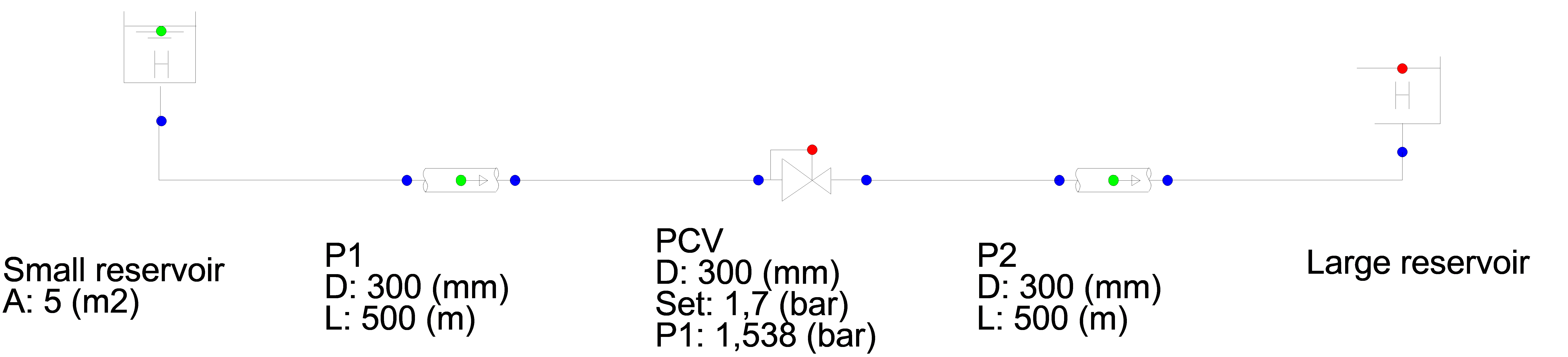
Fig. 4.10.10 Schematic overview of the Wanda model

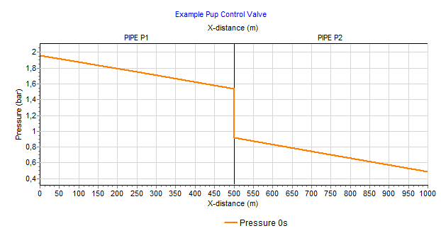
Fig. 4.10.11 Pressure over x-distance for pipe P1 and P2

In the unsteady state the PuCV starts controlling. Due to the decreasing pressure in the small reservoir the PuCV adjusts the position continuously to maintain the set pressure (1.7 bar).

At T= 200 sec, the setpressure has been changed to 1.4 bar (via the action table).

Next figure shows the results.

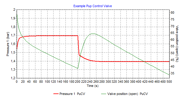
Fig. 4.10.12 Pressure and valve position over time for pressure control valve (PuCV)