4.32. Turbine

4.32.1. Turbine (class)

Fig. 4.32.1 Turbine component

Turbine with adjustable vanes

Fall type

type label	description	active
Turbine	A turbine whose speed is controlled by its vane position, absorbed power and upstream/downstream hydraulic conditions.	yes

The turbine is an active Fall-type component. It is controlled by its vane position, the power absorbed by the electricity grid and the upstream/downstream hydraulic conditions.

Notes:

1. The absorbed power must be less than the maximum available hydraulic power ( \(\rho g Q H \eta\) ) at all times.

2. A hydraulic system based on BoundH boundary conditions is recommended. Otherwise, convergence problems can be encountered with a BoundQ boundary condition (i.e., multiple solutions could exist for the hydarulic system).

4.32.1.1. Mathematical model

The governing equations of the turbine are:

Continuity

(4.32.1)\[Q_{1}=Q_{2}\]

Head balance

(4.32.2)\[H_{1}-H_{2}=H(Q, N, Y)\]

Torque-speed

(4.32.3)\[T(Q, N, Y) N-P_{a b s}=I_{p} N \frac{d N}{d t}\]

with,

Symbol	Description	SI-units
\(Q_{1}\)	upstream discharge	[m3/s]
\(Q_{2}\)	downstream discharge	[m3/s]
\(H_{1}\)	upstream head	[m]
\(H_{2}\)	downstream head	[m]
\(H(Q, N, Y)\)	Head loss across the turbine	[m]
\(T(Q, N, Y)\)	Torque generated by the turbine	[Nm]
\(N\)	Turbine speed	[rad/s]
\(Y\)	Turbine vane position	[rad]
\(T N\)	Power generated by the turbine	[W]
\(P_{a b s}\)	Power absorbed by the power grid	[W]
\(I_{p}\)	Turbine polar moment of inertia	[kg.m2]
\(t\)	time	[s]
\(\rho\)	Actual fluid density (entered in fluid specifications window)	[kg/m3]
\(\rho_o\)	Reference fluid density (typically 1000 for water of 4 °C)	[kg/m3]

4.32.1.2. Turbine data curves

The turbine headloss \(H(Q, N, Y)\) and torque \(T(Q, N, Y)\) need to be determined from the governing equations. The headloss and torque are calculated from the data provided by the manufacturer, using the following relationships:

(4.32.4)\[Q(H, N, Y)=Q_{11}\left(N_{11}\right) D^{2} \sqrt{H}\]

with

(4.32.5)\[N_{11}=\frac{N D}{\sqrt{H}}\]

with the unit value curve for the discharge \(Q_{11}\left(N_{11}\right)\), the unit value curve for the torque \(T_{11}\left(N_{11}\right)\), and the reference diameter D.

The \(Q_{11}\left(N_{11}\right)\) and \(T_{11}\left(N_{11}\right)\) unit value curves do usaully not allow for accurate interpolation of an arbitrary vane position. Improved interpolation is achieved by transforming the unit value curves into \(Q_{11}\left(N_{11} \quad y / y_{\max }\right)\) and \(T_{11}\left(N_{11} y / y_{\max }\right)\) curves. The Wanda turbine component computes these transformed unit value curves from two .trb input files, which contain a set of interpolation curves.

Notes:

• ymax­ is a reference value, hence the dimensionless y/ymax may be > 1.

• The unit curves \(Q_{11}\left(N_{11}\right)\) and \(T_{11}\left(N_{11}\right)\) need to be supplied with an ordered set of \(N_{11}\) values per vane position (\(y\)).

Figure 1.1 presents an example set of transformed unit value curves. For a fixed head drop, vane position, diameter and speed, the discharge and torque can be found.

For example:

Variable	Value
speed	N = 600 rpm
reference diameter	D = 1590 mm
head drop	H = 350 m
relative vane position	y/ymax = 1 (100%)

yields: \(N_{11}=\frac{N D}{\sqrt{H}}=51 \mathrm{rpm} \cdot \mathrm{m}^{1 / 2}\) and then from Figure 1.1: Q₁₁ = 0.224 m^½/s and T₁₁ = 370 N/m³ and with equations 4 and 5: Q = 10.6 m³/s and T = 521 kNm.

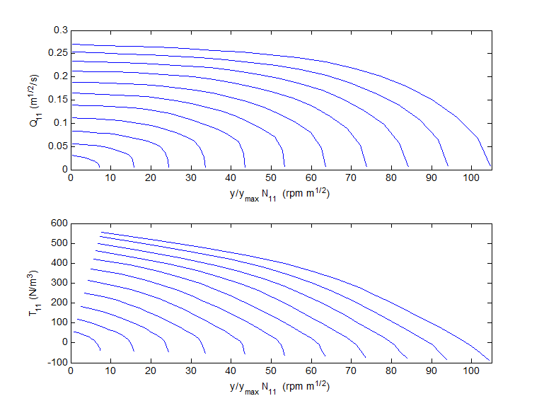
Fig. 4.32.2 Example turbine unit value curves

References

1. E.B. Wylie, V.L. Streeter, “Fluid Transients”, McGraw-Hill, New York, 1978.

2. A.P.Boldy, N.Walmsley “Representation of the characteristics of reversible pump turbines for use in waterhammer simulations”, Paper G1, Fourth Int. conference on Pressure Surges, University of Bath, England, September 21-23, 1983

3. C.S. Martin, “Transformation of pump-turbine characteristics for hydraulic transient analysis”, Proceedings, Eleventh Symposium of the section on Hydraulic Machinery, Equipment and Cavitation, IAHR, Amsterdam, 1982, Paper 30

4.32.2. Turbine model

4.32.2.1. Hydraulic specifications

Description	Input	SI-unit	Default	Remarks
Turbine file nr	Real	[-]	1	Reference number for the turbine input data (.trb) files: CASE_###T11.trb and CASE_###Q11.trb. See below.
Reference diameter	Real	[m]		Turbine diameter related to the unit value curves in the input files.
Polar moment of inertia	Real	[kg.m2]		Moment of inertia.
Rated head	Real	[m]		Rated (or nominal) head, used for start vector in solution process.
Prescribed relative vane position	Table			Relative vane position y/ymax as function of time.
Initial power absorbed	Real	[W]		Power absorbed by the electricity grid at t=0 s.
Initial speed	Real	[rad/s]		Speed at t=0. A realistic value should be used (see below).
Action table	Real	[W]		The absorbed power can be changed using this time-power action table.

NOTE: Turbine file format

The ‘interpolation curves’ in the turbine data files can be used to determine the values of \(Q_{11}\left(N_{11} \quad y / y_{\max }\right)\) and \(T_{11}\left(N_{11} y / y_{\max }\right)\) or to reconstruct the unit value curves for an arbitrary vane position. The data files contain the number of vane positions and an array of vane positions in the header and the number of interpolation curves and the actual interpolation curves (x and y values) in the body. Rows starting with ‘*’ are ignored.

The file name consists of the CASENAME, the number specified in the input field, Q₁₁ or T₁₁ and the .trb extension. The interpolation curves are sorted from lower \(N_{11} y / y_{\max }\) values at the top of the file to higher values at the bottom.

The interpolation curves define the points for each vane position. Therefore, the number of columns for each curve is the same as the number of vane positions. Each curve has a row for \(N_{11} y / y_{\max }\) [rpm.m^1/2] and a row for \(Q_{11}\) [m^1/2/s] or \(T_{11}\) [N/m³] corresponding to the actual vane positions. Please note that the units of \(N_{11}\) in the turbine files are defined as [rpm.m^1/2], which is not conform the SI-unit standard.

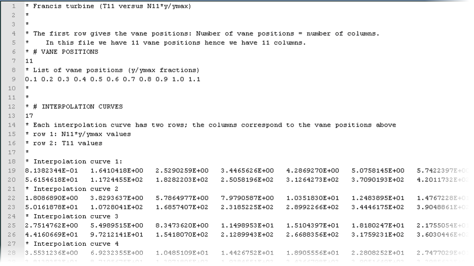
Fig. 4.32.3 Example of a part of the input file “Turbine_001T11.trb”

NOTE: Initial speed

An estimate of the initial speed should be given such the generated and absorbed power are in equilibrium at t=0s. The equilibrium initial speed can be found through trial-and-error calculation where hydraulic conditions, vane position and absorbed power are kept constant during the simulation. By plotting the turbine speed in time series, the equilibrium speed can be identified. However, multiple solutions exist. The user has to check whether the Generated Power equals the Absorbed Power. The right equilibrium speed must result in the turbine generated power being equal to the absorbed power at t=0.

4.32.2.2. Component specific output

Description	SI-unit	Remarks
Turbine speed	[rad/s]	Rotational speed of the turbine
Relative vane position	[-]	Relative position (y/ymax) of the vanes
Power generated	[W]	Power generated by the turbine
Power absorbed	[W]	Power absorbed by generator / electricity grid
Torque generated	[Nm]	Torque generated by the turbine
Torque absorbed	[Nm]	Torque absorbed by the generator
N11	[rpm.m1/2]	Transformed turbine speed (in rpm Instead of rad/s)
Q11	[m1/2/s]	Transformed turbine discharge
T11	[N/m3]	Transformed turbine torque

4.32.2.3. H-actions

The turbine component differs from other components regarding H-actions. Although for most components the H-action controlled by the control signal line is the same as what can be controlled through an action table, the turbine has two different H-actions:

• Action table: changes the absorbed power

• Control signal line: changes the vane position

4.32.2.4. Component messages

Message	Explanation
\(\rho g Q H \eta\) Warning: Could not solve head for given discharge and speed.	Unable to compute a head from the Q11/T11 turbine files (.trb), based on the present discharge and speed.
Warning: N11*y/ymax below turbine data range	Computed N11*y/ymax value is less than the minimum value in the Q11/T11 turbine files (.trb)
Warning: N11*y/ymax above turbine data range	Computed N11*y/ymax value is larger than the maximum value in the Q11/T11 turbine files (.trb)
Error: Input file not found	The turbine data files: CASENAME_###T11.trb and/or CASENAME_###Q11.trb could not be found.
Error: Input file already in use by other RDFILE	The turbine data file is already in use by another turbine component.
Error: Error with input file	The data in the turbine input file contains an error
Error: Error in turbine file	The data in the turbine input file contains an error
Error: decrease NVANES	Number of vanes used in turbine data file is greater than the maximum number of vanes allowed in WANDA (20).
Error: decrease NCURVES	Number of ‘interpolation curves’ used in the turbine data file is greater than the maximum number of ‘interpolation curves’ allowed in WANDA (20).
Error: Inconsistent initial vane position at t=0s and input of control system	The initial control system value and the initial vane position specified by the user are different.
Error: Control system gives negative vane position	Only positive vane positions are allowed.

4.32.3. Examples

4.32.3.1. Model description

The following example is meant to explain the function of the turbine component. The turbine is placed between two reservoirs, as shown in Figure . As this example is an academical case, the pipeline systems at both sides of the turbine are neglected. However, in practical applications the influence of the pipeline should be considered (see example 2).

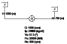
Fig. 4.32.4 Wanda scheme.

The turbine interpolation curves are saved in the example files Turbine_001T11.trb and Turbine_001Q11.trb. Figure presents a visual representation of these curves. In addition, the unit curves have been reconstructed from the interpolation curves and have also been added to the figure.

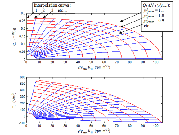
Fig. 4.32.5 Turbine unit curves with interpolation curves (see example directory for the input files “Turbine_001T11.trb”and “Turbine_001Q11.trb”)

4.32.3.2. Finding the equilibrium speed for a specified P_abs

The following procedure can be followed to find the speed that places the generated power in equilibrium with the absorbed power: An initial speed equal to the rated speed is input (for this example 600 rpm) and a transient calculation performed without varying the hydraulic conditions, vane position or absorbed power. Figure shows that the absorbed power and generated power are not in equilibrium with an initial speed of 600 rpm. For the next 35s the turbine speeds up in order to balance the absorbed and generated power. After 35s the turbine has reached an equilibrium with a speed of approximately 751.6 rpm. This equilibrium speed can be used in subsequent transient calculations, where the turbine is initially in equilibrium.

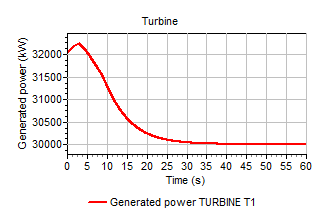
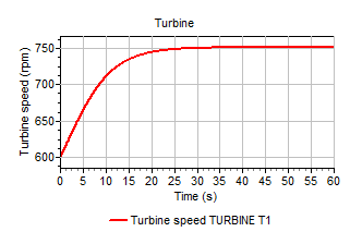
Figure 1.5. Turbine speed increases as power is not in equilibrium at t=0s.

4.32.3.3. Varying the absorbed power P_abs

At t=0s there is an equilibrium between generated and absorbed power. The absorbed power is lowered from 30000 at t=20s to 25000 kW at t=40s (using the action table of the turbine). Due to the inertia of the turbine a disequilibrium will develop. The turbine will speed up in order to lower the generated power and to restore the equilibrium. Figure shows the increase of the turbine speed at constant vane position.

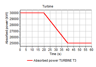
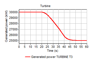
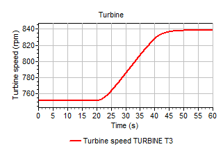
Fig. 4.32.6 Decreasing power results in increasing turbine speed.

4.32.3.4. Varying the vane position

By changing the vane position, it is possible to control the speed of the turbine. A control signal line is connected to the turbine as shown in Figure . It is also possible to vary the vane position with the table property. If both the control table and the property table are present, the control table will prevail. The signal decreases the vane position from 100% of the maximum angle at t=5s to 95% at t=25s. For this example the absorbed power is kept constant (P_abs = 30 000 kW).

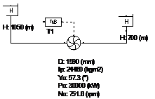
Fig. 4.32.7 Wanda scheme and connection of signal line.

The system is in equilibrium at t=0s. The discharge and generated power will decrease due to the decreasing vane position, as can be expected from the turbine unit curves. Figure 1.8shows the generated power and the vane position. After t=25s the vane position is kept constant.

Due to the imbalance between generated and absorbed power the speed of the turbine changes. Because the generated power is lower than the absorbed power, the speed of the turbine is decreasing according to equation 3. At t=60s the turbine is in equilibrium again as the speed is constant and the generated power equals the absorbed power.

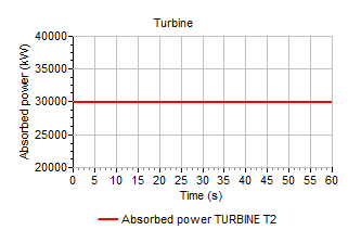
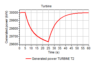
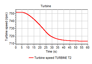
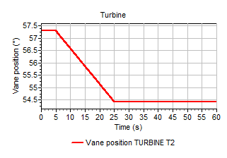
Figure 1.8. Changes in generated power due to reduced vane position.

4.32.3.5. More realistic example

To show the influence of the pipeline system on the turbine a more realistic case is included as well. Here the absorbed power is initially in equilibrium at 27970 kW. At t=10s the absorbed power drops to 22000 kW at t=30s. The vane position is reduced to prevent too high speed values. Since the change of vane position is a reaction to the drop in absorbed power, the vane position changes with a delay of 5 seconds from 100% (at t=15s) to 76% (at t=35s). Figure 1.9 shows the scheme for this example including the pipelines.

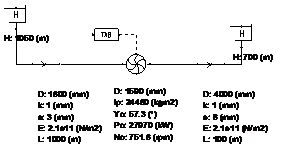
Fig. 4.32.8 Wanda scheme

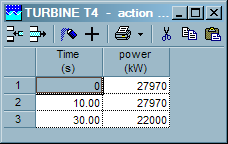
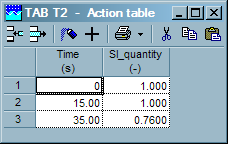
Figure 1.10: Input via action table (left) and control-table (right)

Figure 1.11 shows the change in power, speed and vane position. Due to the inertia there is a ‘overshoot’: the generated power drops below the equilibrium value when the absorbed power is kept constant again (at t=30s). At t=50 the system is in equilibrium again.

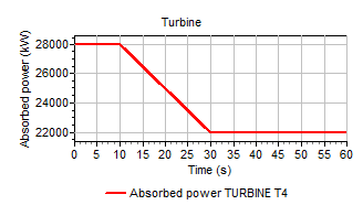
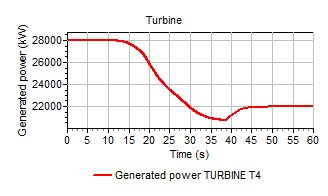
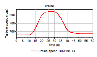
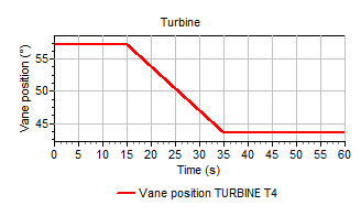
Figure 1.11: Power, speed and vane position

It is of course also possible to build a control system with a sensor to measure the pump speed and feeding this into a PID controller which feeds the vane position back into the turbine.