4.9. Conduit

Fig. 4.9.1 Conduit

Fall type

type label	description	active
Free surface flow conduit	Pipe model for free surface (atmospherically) flow and pressurised flow without waterhammer calculation	No

The free surface conduit is capable of simulating the behaviour of free surface phenomena. The application of this component is useful for simulation of slow filling and draining procedures.

The free surface conduit is capable of handling circular cross sections or arbitrary cross sections defined by a table.

4.9.1. Free surface flow conduit

4.9.1.1. Mathematical model

The dynamic behaviour of a free surface pipe is described by the continuity and momentum equation.

The mathematical model is described in chapter “Free surface flow conduit” on page 184.

A summary of the relevant aspects for the user with respect to the input are repeated in this section.

It is assumed that the gas (air) above the free surface in this pipe or channel can enter or leave the pipe freely without causing pressure surges.

The applicability of the continuity and momentum equations for free-surface flow (Saint-Venant equations) is limited to slopes of 1:7 (8 degrees or 14%).

In addition to the maximum slope, the slope change in two consecutive free surface elements is limited. The maximum slope change should be less than 0.14. Formally:

The element length of free surface pipes is calculated from the time step. However in Engineering mode the time step is not present. Therefore the user should specify explicitly a maximum element length, which is used in Engineering mode. It is recommended to set this property to 200*D (diameter) or less. In Transient mode the element length is calculated from the time step and it is checked whether the calculated element length is less than the maximum element length. It is recommended to set the maximum element length to 200*D or less, in order to obtain sufficient accuracy.

4.9.1.2. Geometry

Each CONDUIT must have a length input and height location. This so-called profile can be defined in several ways:

1. Scalar value for length

2. Length-height profile

3. Isometric layout specified with absolute XYZ co-ordinates

4. Isometric layout specified with differential XYX co-ordinates.

Each type of profile input is translated to a longitudinal profile (X-H profile). In case of a scalar value the height of the beginning and the end of the conduit is derived directly from the adjacent H-nodes. The input height is the height of the bottom (!) of the conduit, as indicated in figure below. Note that the pressurised pipe uses the centre line for elevation reference.

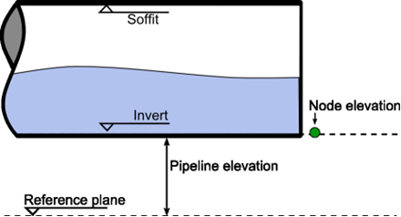
Fig. 4.9.2 Definition of the height of the Conduit and the node elevation.

The CONDUIT use the same geometry profile type as used in the PIPE, For details see the PIPE component.

4.9.1.3. Hydraulic specifications

description	Input	unit	default	remarks
Cross section	Table Circle	[-]	Circle
Height-width table				if cross section=Table
Inner diameter	real	[m]		if Cross section=Circle
Initial flow condition	Qinit > 0 Qinit = 0		Qinit>0	if Cross section=Rectangle
Drained	Complete Offtakes		Complete	if Initial flow condition = Qinit=0 See additional remark
Offtake locations	Table			If Drained =offtakes See additional remark
Friction model	D-W k D-W f	[-]	D-W-f	Darcy Weisbach friction model with wall rougness or friction factor input
Wall roughness	real	[m]		If friction model = D-W k
Friction factor	real	[-]		If friction model = D-W f
Dynamic friction	none Quasi-steady		Quasi-steady	Only If friction model = D-W k
Max. element length	real	[m]
Geometry input	Length l-h xyz xyz diff	[-]
Length	real	[m]		if Geometry input = Length
Profile	table			if Geometry input = L-h, xyz or xyz diff

Remarks Initial flow condition / drained

Contrary to the “initial flow condition: Qinit > 0” the “initial flow condition: Qinit = 0” ipe is intended to compute steady states with zero flow and an arbitrary filling status. With zero flow there may exist pools of liquid around the deep points in the pipe profile. In how far the pipe will be drained is specified by the user input item “drained”. This property can either be “complete” (pipe will be completely empty) or “offtakes” in which case offtake locations where the pipe will be drained are specified. The offtake locations are specified by means of a 3-column table in which the first two columns correspond to the profile table of the pipe (lines may be skipped, however). Offtake locations will be active when there is a positive non-zero entry in the third column at the station required. They are inactive when there is either a zero or an empty field in the third column. The offtake level will be the bottom elevation of the pipe (i.e. profile elevation minus pipe height: diameter or highest table entry).

For instance a 4 m diameter conduit with profile:

X	Z
0	50
1000	35
2000	40
3000	30
4000	45
5000	35
6000	45

and offtake table:

X	Z	offtake
0	50	0
3000	30	1
6000	45	0

will have the following solution:

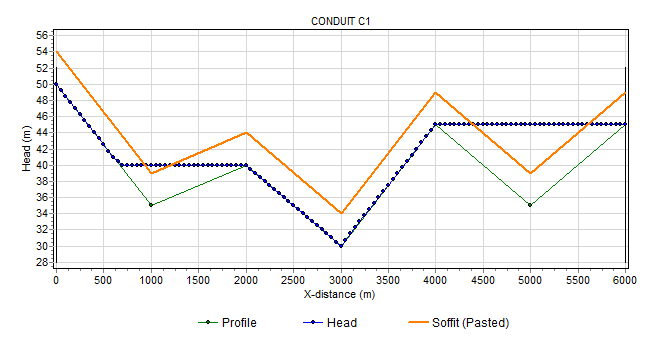
Fig. 4.9.3 Solution of the conduit C1 showing head over x-distance.

Note: the soffit line is not standard output but pasted from a spreadsheet (elevation soffit = profile points + diameter)

4.9.1.4. Component specific output

Output	Description
Froude [-]	Froude number
Depth [m]	fluid depth related to bottom
Level [m]	fluid level related to horizontal reference plane

4.9.1.5. H-actions

None

4.9.1.6. Example

None