4.39. X-JUNCTION
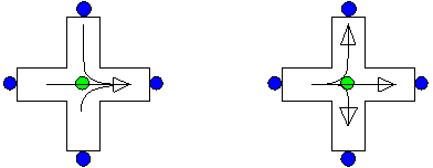
Fig. 4.39.1 X-Junction
type label |
description |
active |
|---|---|---|
X-junction (merging) |
Four-node junction with rectangular legs and a merging flow. Both straight legs have the same diameter |
no |
X-junction (dividing) |
Four-node junction with rectangular legs and a dividing flow. Both straight legs have the same diameter |
no |
Both components supports only a “3-flow” merging and dividing flow in the positive and negative main flow direction (from connect node 1 to 2 or vice versa).
The merging type supports the dividing flow regime and the dividing type supports the merging flow regime
4.39.1. Mathematical model
4.39.1.1. Positive flow definition
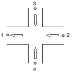
The definition for the positive direction of flow (and velocity) is important to understand the results in the property window. Each X-junction type has his own definition. The arrows in the symbol specify the positive direction of the flow (and the velocity).
For the X-junction (merging) component the positive flow definition is defined in the left figure below.
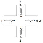
Fig. 4.39.2 X-junction (merging).
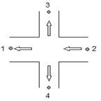
For the X-junction (dividing) component (right figure) the positive flow definition for the branch leg is opposite to that of the Y-junction combining. The positive flow definitions in the main legs (1 to 2) are the same for both types.
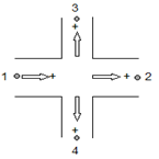
Fig. 4.39.3 X-junction (dividing).
4.39.1.2. Flow regimes
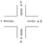
In the table below all supported flow regimes are listed and explained with a scheme with corresponding actual flow arrows.
For all other not supported flow regimes the local losses in the X-junction will be ignored, that means the component is frictionless.
1 Combining flow |
Positive flow |
Negative flow |
|---|---|---|
2 Dividing flow |

Positive flow |
Negative flow |
4.39.1.3. Equations
The head loss over a 4-node component depends on the distribution of the discharges and the area of the connected legs. The X-junction supports only the resistance coefficient Xi (ξ) according the head loss functions of Idelchik’s Handbook
Please note that the loss coefficients according to the handbooks apply to junctions with a certain minimum pipe length interval in between multiple junctions.
The head loss in 4-node components is a function of the combined flow in the combined leg, which is either one leg (1 or 2) of the straight part. Including the continuity equation (no production or loss of mass in the component) the general set of the four equations of the X-junction is:
X-junction merging
ΔH X-junction merging, combined flow in leg 2
X-junction dividing
ΔH X-junction dividing, combined flow in leg 1
Where: Q i = total discharge in leg i [m3/s]
Hi = energy head in connect point i [m]
Ai = pipe area leg i (leg with total flow) [m2]
ξij = loss coefficient between point i and j [-]
The subscripts (1), (2), (3) and (4) correspond to the different legs. The subscript x at the discharge Qx refers always to the leg in which the combined (total) flow Q occurs.
For positive dividing flow and negative merging flow, Q1 will be taken into account. For positive merging flow and negative dividing flow, Q2 will be taken into account.
4.39.1.4. Resistance coefficients based on formulas
The resistance coefficients based of formulas are taken from the Idelchik Handbook with the following restriction to the section areas:
The formulas are only valid for the supported flow regimes as explained in table 1. For each formula the ξ‑values for various area and discharge ratios are collected in a table. Note that all indices used in the formulas are based on positive flow.
For the other flow regimes the resistance coefficient can not be retrieved and a ξ=0 will be applied .
X-junction merging
For the straight leg, the resistance coefficient ξ12 is calculated according to:
The table below shows the ξ12values according the formula above for several discharge ratios
Q1/Q2 |
0.0 |
0.1 |
0.2 |
0.3 |
0.4 |
0.5 |
0.6 |
0.7 |
0.8 |
0.9 |
1 |
|---|---|---|---|---|---|---|---|---|---|---|---|
ξ12 |
1.20 |
1.19 |
1.17 |
1.12 |
1.05 |
0.96 |
0.85 |
0.72 |
0.56 |
0.39 |
0.20 |
For the both branch legs, the resistance coefficient is calculated according to:
The subscript i is for the interested branch leg, while j is for the other branch leg.
The table below shows some ξi2values according the formula above for several discharge ratios and area ratios
Qj/Qi |
Qi/Q2 |
||||||
|---|---|---|---|---|---|---|---|
0.00 |
0.1 |
0.2 |
0.3 |
0.4 |
0.5 |
0.6 |
|
Ai/A2= 0.2 |
|||||||
0.5 |
-0.999 |
-0.25 |
0.94 |
2.57 |
4.62 |
7.10 |
9.97 |
1 |
-0.999 |
-0.097 |
1.200 |
2.874 |
4.900 |
7.250 |
- |
2 |
-0.999 |
0.191 |
1.624 |
3.224 |
- |
- |
- |
Ai/A2= 0.4 |
|||||||
0.5 |
-0.999 |
-0.439 |
0.191 |
0.881 |
1.624 |
2.409 |
3.224 |
1 |
-0.999 |
-0.285 |
0.450 |
1.186 |
1.900 |
2.563 |
- |
2 |
-0.999 |
0.003 |
0.874 |
1.537 |
- |
- |
- |
Ai/A2= 0.6 |
|||||||
0.5 |
-0.999 |
-0.474 |
0.051 |
0.566 |
1.064 |
1.535 |
1.966 |
1 |
-0.999 |
-0.320 |
0.310 |
0.872 |
1.341 |
1.689 |
- |
2 |
-0.999 |
-0.032 |
0.734 |
1.222 |
- |
- |
- |
Ai/A2= 0.8 |
|||||||
0.5 |
-0.999 |
-0.486 |
0.003 |
0.459 |
0.874 |
1.237 |
1.537 |
1 |
-0.999 |
-0.332 |
0.263 |
0.764 |
1.150 |
1.391 |
- |
2 |
-0.999 |
-0.044 |
0.686 |
1.115 |
- |
- |
- |
Ai/A2= 1 |
|||||||
0.5 |
-0.999 |
-0.491 |
-0.019 |
0.408 |
0.784 |
1.096 |
1.334 |
1 |
-0.999 |
-0.337 |
0.240 |
0.714 |
1.060 |
1.250 |
- |
2 |
-0.999 |
-0.049 |
0.664 |
1.064 |
- |
- |
- |
X-junction dividing
For the straight passage the resistance coefficient is:
where Qbr is the mean discharge in the branches (i.e. 0.5*(Q3 + Q4) ) and τ1 depends on the area and discharge ratios as given in the table below.
For the branch legs there are two cases, depending on area ratio:
For Ai/A1 ≤ 2/3
For Ai/A1 = 1 (up to vi/v1 ≈ 2.0)
where the values of A’ are taken from table 6.
As an example some values for the resistance coefficients ξ12 and ξ1i are given in the tables below, depending on the section area and discharge ratios.
\(Q_2/Q_1\) |
ξ12 |
||
|---|---|---|---|
0.1 |
0.004 |
-0.016 |
- |
0.2 |
0.016 |
-0.024 |
- |
0.3 |
0.036 |
-0.024 |
- |
0.4 |
0.064 |
-0.016 |
- |
0.5 |
0.100 |
0.000 |
- |
0.6 |
0.144 |
- |
0.036 |
0.7 |
0.196 |
- |
0.084 |
0.8 |
0.256 |
- |
0.144 |
0.9 |
0.324 |
- |
0.216 |
1 |
0.400 |
- |
0.3 |
4.39.2. X-Junction properties
The input and output properties of both X-junction are exactly the same.
4.39.2.1. Properties X-junction (merging and dividing type)
Description |
input |
unit |
range |
default |
Remarks |
|---|---|---|---|---|---|
Diameter straight leg |
Real |
[mm] |
D leg 1 = D leg 2 |
||
Diameter branch leg |
Real |
[mm] |
D leg 3 = D leg 4 |
Component specific output X-junction (merging and dividing)
Loss coefficient straight [-] |
The ξ12 for positive flow and ξ21 for negative flow |
|---|---|
Loss coefficient branch 1 [-] |
The ξ13 for positive flow and ξ31 for negative flow |
Loss coefficient branch 2 [-] |
The ξ14 for positive flow and ξ41 for negative flow |
Head loss straight [m] |
The ΔH12 for positive flow and ΔH21 for negative flow |
Head loss branch 1[m] |
The ΔH13 for positive flow and ΔH31 for negative flow |
Head loss branch 2 [m] |
The ΔH14 for positive flow and ΔH41 for negative flow |
Component messages Y-junction (combining and dividing)
Message |
Type |
Explanation |
|
|---|---|---|---|
Merging |
Info |
Positive straight flow |
Negative straight flow |
|
|
||
Dividing |
Info |
Positive straight flow |
Negative straight flow |
|
|
||
Not supported flow regime |
Info |
Other flow regimes; ξ=2.0 |
NOTE: The numbering of the branches in the literature is not always consistent with the WANDA definition as given under ‘Mathematical Model’ above.