4.8. Collector¶

4.8.1. Collector (class)¶

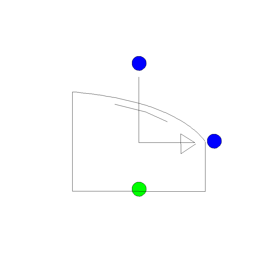
../_images/image427.png — Fig. 4.8.1 Short open channel with constant slope and lateral inflow¶

Fall type

type label	description	active
Collector	Short open channel with constant slope and lateral inflow	no

Note: In transient mode, this component computes a steady-state profile for each time-step.

4.8.1.1. Mathematical model¶

The collector model is used for (increasing) spatially-varied flow problems. It is used to compute the upstream and downstream flow depths and velocities in a channel with constant slope (-8° to +8°, or -14% to +14%). Figure 1 presents the definition sketch of the collector model. The collector is closed at the upstream end and the lateral inflow is distributed uniformly along the length of the collector. The hydraulic control from which the upstream flow depth is computed can be inside the collector or at the downstream end. If the control is at the downstream end then it is assumed that the flow is either critical or subcritical. The collector does not account for the occurrence of a hydraulic jump (which might occur when the hydraulic control is between the upstream and downstream boundaries and the downstream boundary has a subcritical flow depth). Furthermore, the flow out of the collector always occurs at the downstream end and never laterally ().

The geometry of the collector cross-section can be specified by the user using a depth-width table or simply by selecting a rectangular or half-round shape. Furthermore, the channel cannot overflow when the calculated flow depth exceeds the last entered depth-width table entry, since the model uses the last depth-width entry for such situations. Finally the model does not support dry channel situations (zero flow depth).

The depth profile along the length of the collector is curved for the following reasons:

The flow velocity and head loss increases due to the lateral inflow.
The lateral inflow introduces large local losses near the upstream end of the collector.
The lateral inflow has no impulse in the streamwise direction.

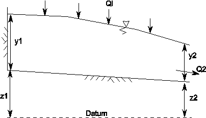
../_images/image428.png — Fig. 4.8.2 Definition sketch of collector¶

Flow profile computation

The flow profile (and ultimately the upstream flow depth ) is computed from

(4.8.1)¶\[\frac{d y}{d x}=\frac{S_{0}-S_{f}-\frac{2 \alpha Q q^{*}}{g A^{2}}}{1-\frac{\alpha Q^{2}}{g A^{2} D}}\]

with:

Variable	Description	Units
\(S_0\)	Bed slope	-
\(S_f\)	Friction slope	-
\(\alpha\)	Energy coefficient	-
\(Q\)	Discharge	m³/s
\(q\)	Lateral discharge per unit length	m³/s
\(g\)	Gravitational acceleration	m/s²
\(A\)	Cross-sectional area	m²
\(D\)	Hydraulic depth	m

(4.8.1) is solved using the direct-step method. T he computation starts at a known downstream depth. A default depth is assumed for the following upstream point and its slope is computed from equation (4.8.1). If the slopes of the upstream and downstream points do not differ by more than 1%, then the computation proceeds to the next upstream point. If the two slopes differ by more than 1% then the default depth of the upstream point is adjusted. Its slope is recomputed and again compared to the slope of the downstream point.

Hydraulic control

In order to use (4.8.1) a known downstream flow depth is required. The computation proceeds upstream from this known depth, assuming subcritical flow.

The known flow depth is determined as follows:

The algorithm first checks to see whether a hydraulic control occurs between the upstream and downstream boundaries of the collector. The location and flow depth of this hydraulic control is determined from a singular point analysis [1,2]. If the there is such a hydraulic control then. If no hydraulic control occurred between the upstream and downstream boundaries, then the computation starts at the downstream boundary. At the downstream boundary the flow depth is the maximum of: the critical depth (free overfall), the uniform flow depth (if specified by the user) or the head of the downstream hydraulic node.

The critical flow depth yc is determined from

(4.8.2)¶\[y_{c}=\frac{Q_{2}^{2}}{A_{2}^{2}\left(y_{c}\right) \cdot g} \quad F r=\frac{Q_{2}}{A_{2} \sqrt{g \cdot y_{c}}}\]

The uniform flow depth yn is determined from

(4.8.3)¶\[Q=A\left(y_{n}\right) \cdot C \sqrt{R_{h}\left(y_{n}\right) \cdot S_{b}}\]

with:

Variable	Description	Units
\(y_c\)	Critical flow depth	m
\(y_n\)	Uniform flow depth	m
\(Fr\)	Froude number	-
\(Q\)	Discharge	m³/s
\(C\)	Chezy friction factor	m^0.5/s
\(g\)	Gravitational acceleration	m/s²
\(A\)	Cross-sectional area	m²
\(R\)	Hydraulic radius	m
\(S_b\)	Bed slope	-

The equations are solved iteratively. The Chezy friction factor (\(C\)) is computed from:

(4.8.4)¶\[C=\sqrt{\frac{8 g}{f}}\]

The Colebrook-White friction factor (\(f\)) is defined as:

(4.8.5)¶\[\frac{1}{\sqrt{f}}=-2 \log \left(\frac{k / D_{h}}{3.7}+\frac{2.51}{\operatorname{Re} \sqrt{f}}\right)\]

The Reynolds number (\(Re\)) is defined as:

(4.8.6)¶\[\operatorname{Re}=\frac{v D_{h}}{v}=\frac{v 4 R_{h}}{v}\]

with:

Variable	Description	Units
\(k\)	Absolute roughness of the channel	m
\(D_h\)	Hydraulic diamter	m
\(Re\)	Reynolds number
\(v\)	Flow velocity	m/s
\(\nu\)	Kinematic viscosity	m²/s

They are computed at the collector midpoint (L/2).

4.8.2. Collector¶

4.8.2.1. Hydraulic specifications¶

Description	Input	Unit	range	default	remarks
Length	Real	[m]	(0 ; 1000)
Wall roughness	Real	[mm]	(0 ; 1000)
Cross section	rectangular / semi-circular / table			rectangular
Width	Real	[m]	(0 ; 10)		If cross-section is specified as rectangular or semi-circular
Depth-width table	table				If cross-section is specified as table
Upstream bottom offset	Real	[m]	[-140 ; 140]		w.r.t. downstream H-node
Downstream condition	Uniform/ Free overfall

See also “Mathematical model” (Section 4.8.1.1).

Remarks

The upstream and downstream bed levels are equal to the sum of their respective bottom offsets and the downstream H-node geometric height. The slope of the collector bed must be less than 14 % due to constraints of the mathematical model.

The component upstream of the collector should specify a discharge and not a head (a BOUNDQ or WEIR component, for example). The discharge through the collector must be greater than zero (i.e. the collector cannot be drained).

As with the CHANNEL component, the collector does not allow for transitions between sub- and supercritical flow. The component will issue a warning if it detects a hydraulic jump or a transition from subcritical to supercritical flow.

4.8.2.2. Component specific output¶

Description	Unit	remarks
Velocity downstream	m/s
Depth upstream	m
Depth downstream	m
Normal depth downstream	m
Critical depth downstream	m
Froude number downstream	-

4.8.2.3. H-actions¶

None

4.8.2.4. Component messages¶

Message	explanation
Info: Slope horizontal/adverse; normal depth infinite	Bottom offset values, result in a slope which is either horizontal or adverse
Error: Lateral inflow may not be zero.	No discharge is being supplied by component upstream of collector
Info: Critical flow between upstream and downstream boundaries	Hydraulic control occurs between upstream and downstream boundaries
Info: Downstream Froude<=1: Tranquil flow	Flow at downstream end is subcritical. The subcritical flow depth at the downstream boundary is used for the profile computation
Info: Downstream Froude >1: Shooting flow	Flow at downstream end is critical. The critical flow depth at the downstream boundary is used for the profile computation
Terminating Error: Slope > 14%	Slope exceeds 14%. Check elevations of the connected H-nodes.

4.8.2.5. Example¶

The following example demonstrates how to model a settling tank for sewage treatment works.

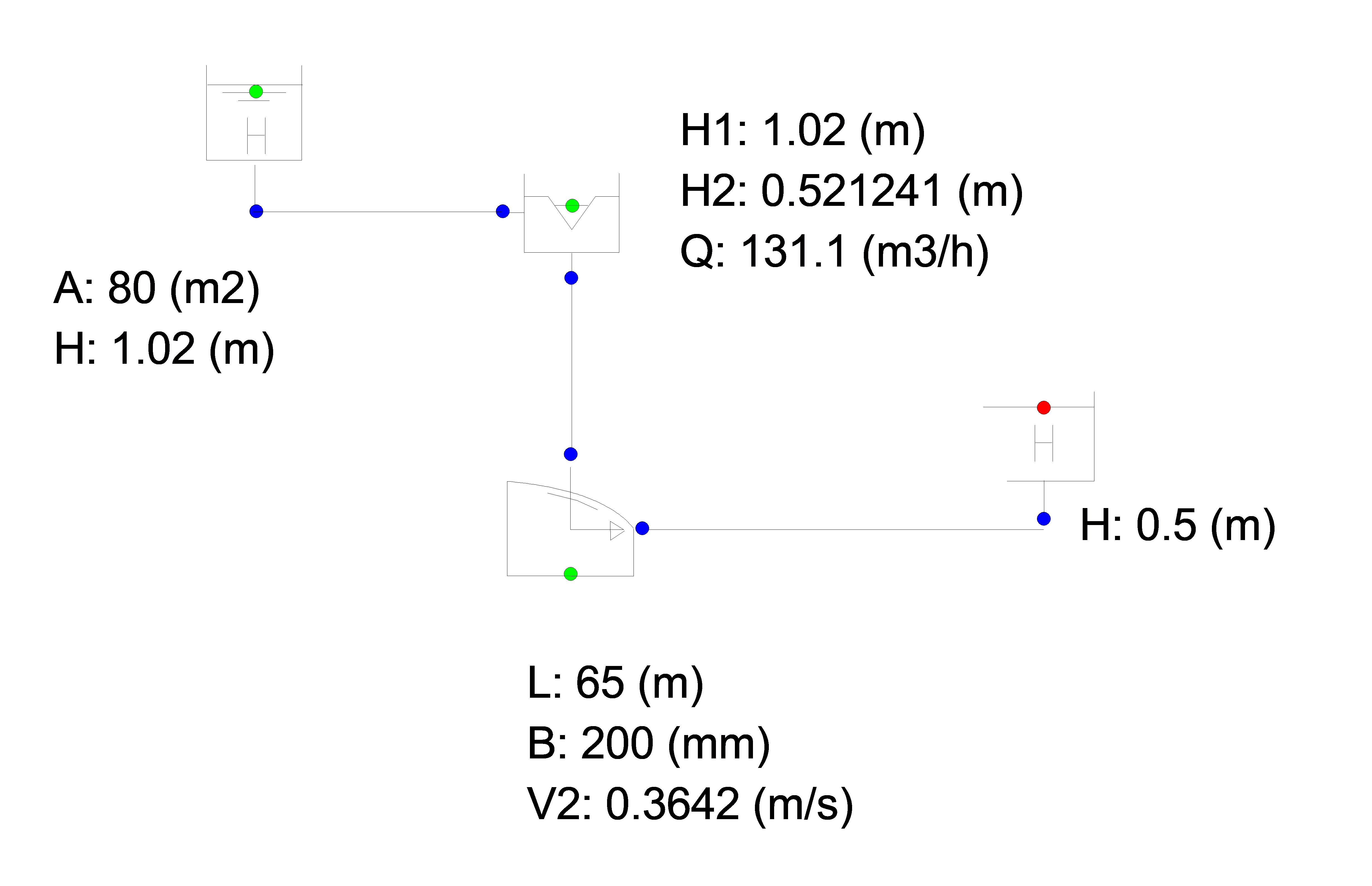
../_images/image435.png — Fig. 4.8.3 Schematic overview of a wanda model.¶

The V-notch weir discharges into the collector. This represents the settling tank overflowing into the surrounding channel.

Literature

V.T. Chow, Open channel hydraulics, Int. ed., McGraw-Hill, Singapore, 1973.
1. Chanson, ‘The hydraulics of open channel flow: an introduction’, Elsevier, Amsterdam, 2004