4.21. Pump Energy

4.21.1. Pump Energy components

A special set H-components are used for the module PumpEnergy. These components are used in combination with the PUMP component. The PumpEnergy components are ignored in the steady and transient calculation.

Overview available components

type	description
PUMPSCEN	Pump operation scenario
Q_PATTRN	Discharge pattern as function of time
Q_FREQ	Discharge frequency in a certain period
SYSCHAR	System characteristic

4.21.1.1. Mathematical model

The PumpEnergy module calculates the total power (kW) of a multi-pumpstation (two or more pumps in parallel arrangement) for a specified operation scenario. If the time is specified the total energy (kWh) is calculated as well. For one or more discharge ranges, the user specify which pumps are running. The running pumps can be speed controlled or fixed speed. If they are speed controlled, the program calculates the speed in such way that the required head (as defined by the given system characteristic) is satisfied.

The pump curves of pumps in parallel placement are summarised. Intermediate points are determined by linear interpolation.

For a certain discharge the point of intersection of the summarised pump curve with the specified system characteristic is computed. In case of variable speed pumps, the affinity rules are used:

(4.21.1)\[\frac{H\left( N_i \right)}{H \left( N_r \right)} = \left( \frac{N_i}{N_r} \right)^{2}\]

(4.21.2)\[\frac{Q\left( N_i \right)}{Q \left( N_r \right)} = \frac{N_i}{N_r}\]

All variable speed pumps are controlled with the same ratio according:

(4.21.3)\[N=N_{\min }+\operatorname{Ratio}\left(N_{\max }-N_{\min }\right)\]

Subsequently the duty point of each individual pump is determined, that means the discharge and head, but also the efficiency and power and, if the duration is known, the energy.

4.21.2. PUMPSCEN (Pump Scenario)

Fig. 4.21.1 Wanda schematic Pump Scenario

4.21.2.1. Input specifications

description	input	unit	range	default	remarks
Scenario	table				See below

The scenario table contains all non-disused pumps available in the diagram.

Q from (m3/h)	Q to (m3/h)	PUMP 1 (rpm)	PUMP 2 (rpm)	PUMP 3 (rpm)
0	1200	0
1200	2400			0
2400	4000		1500	0

For each discharge range (phase) the operating pumps are defined:

• value = 0 (zero) means a variable speed pump

• value > 0 means the actual fixed speed

• empty field means pump is not operating

4.21.2.2. Output specifications

If the pump energy can be computed (depends of Q_PATTRN or Q_FREQ component), the energy consumption for each phase is mentioned in the scenario table. A separate output property is used for the total energy amount.

Q from	Q to	PUMP 1	PUMP 2	PUMP 3	Energy	Energy ratio
(m3/h)	(m3/h)	(rpm)	(rpm)	(rpm)	(MWh)	(%)

The output properties are:

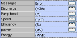
Fig. 4.21.2 Display of the output properties

The message property contains messages with respect to all components use for the PumpEnergy calculation;

Next output properties can be visualised in a chart as function of discharge or time (last one only in combination with Q_PATTRN)

• Discharge

• Head

• Speed

• Efficiency

• Power

In the example the coherence of the Pump Energy components are explained.

4.21.3. Q_PATTRN (discharge pattern)

Fig. 4.21.3 Wanda schematic Pump discharge pattern

4.21.3.1. Input properties

description	input	unit	range	default	remarks
Discharge pattern	table				See below

The discharge pattern table is a 2-columns table

Time (s)	Discharge (m3/s)
Real	Real

Example:

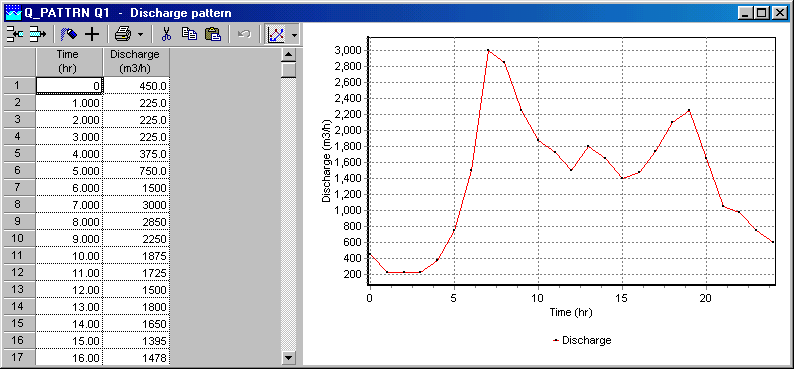
Fig. 4.21.4 Example of discharge pattern

4.21.3.2. Output properties

None

4.21.4. Q_FREQ (discharge frequency)

Fig. 4.21.5 Wanda schematic Pump discharge frequency

4.21.4.1. Input properties

description	input	unit	range	default	remarks
Discharge frequency	table				See below

The discharge pattern table is a 3-columns table; column one and two are used to specify the range, only the second column can be edit; the first column is automatically filled, starting with zero.

Q from (m3/s)	Q to (m3/s)	Time (s)
Real	Real	Real

Example:

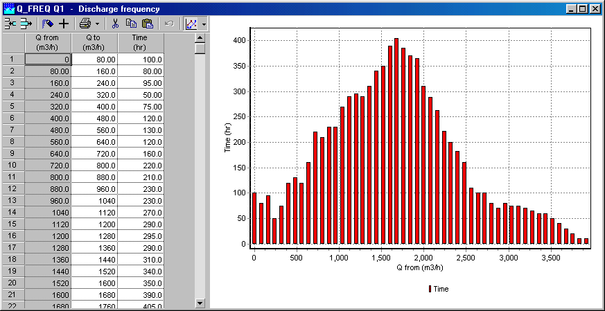
Fig. 4.21.6 Discharge frequency example

4.21.4.2. Output properties

None

4.21.5. SYSCHAR (System characteristic)

Fig. 4.21.7 Wanda schematic system characteristic

4.21.5.1. Input properties

description	input	unit	range	default	remarks
System characteristic	table				See below

The system characteristic is a 2-columns table;

Discharge (m3/s)	Pump head (m)
Real	Real

Example:

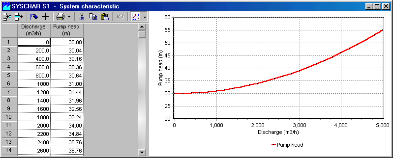
Fig. 4.21.8 Example of the system characteristic table.

The Pump Head is defined as the sum of the static head and dynamic head:

Note: this characteristic can be derived form the System Characteristic module.

See also “System characteristic” (Section 2.14.7)

Create the wanted system characteristic, show the chart and copy the chart data to the clipboard.

Next, copy the chart data into the SYSCHAR table.

4.21.5.2. Output properties

None

4.21.5.3. Example

A pumpstation with three different pumps supplies to a drinking water network. The maximum delivery rate is 4000 m³/h. From history reports the annual delivery ranges are known (see chart given by Q_FREQ)

Note: this example is included in the example directory

The desired pressure in the network (pressure side pump) is defined by the system characteristic:

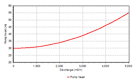
Fig. 4.21.9 Pump discharge versus pump head.

Pumpdata:

Pump id	design capacity (m3/h)	Rated speed curve (rpm)	min speed (rpm)	max speed (rpm)	max power (kW)
1000	1000	1200	1000	1500	150
1300	1300	1200	1000	1500	200
1800	1800	1200	1000	1500	300

The pump curves are given below:

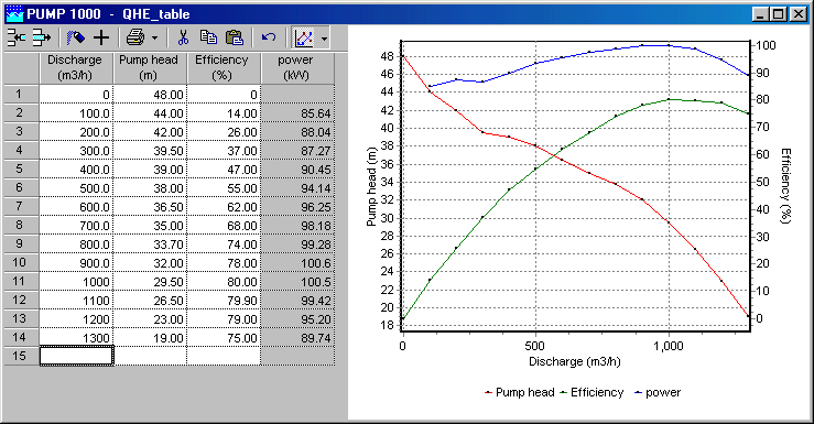
Fig. 4.21.10 Pump curve for pump 10000

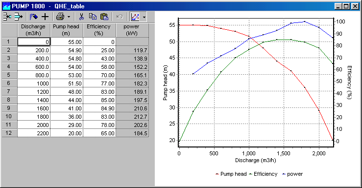
Fig. 4.21.11 Pump curve for pump 1800

Question: Optimise the pump scenario.

Step 1: add components into diagram:

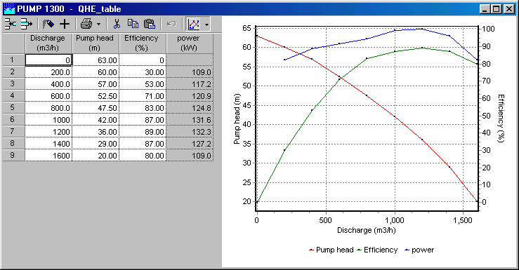
Fig. 4.21.12 Additional pump curve for pump 1300

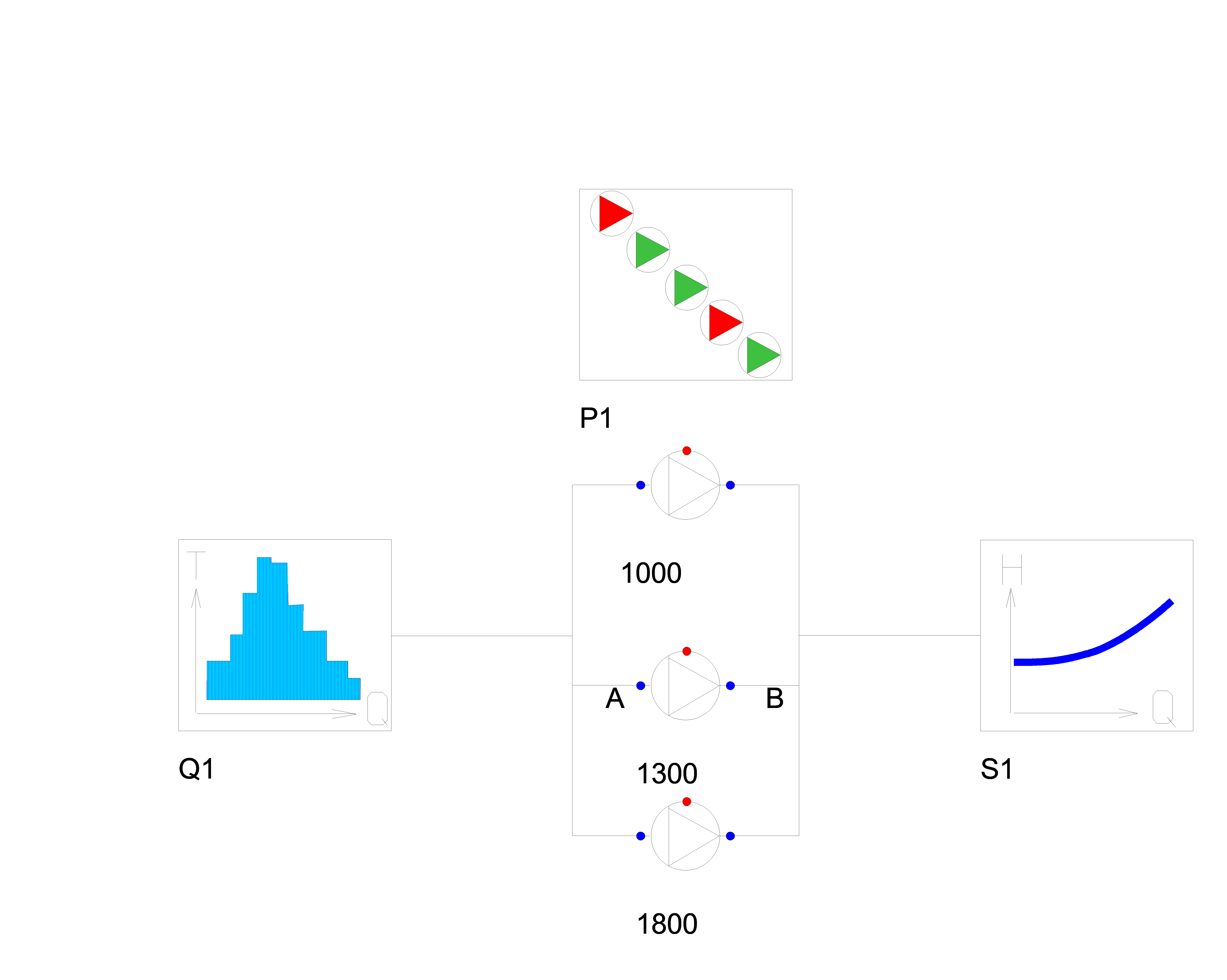
Fig. 4.21.13 Schematic overview of Wanda model.

Step 2: input of pump data and system characteristic

Step 3: choose a scenario

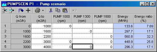
Fig. 4.21.14 Scenario management table

The total energy consumption (annual base according specified frequency) is 1737 MWh

Step 4: analyse the scenario output (especially efficient)

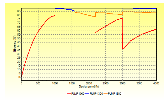
Fig. 4.21.15 Scenario output (graph)

Step 5: adapt the scenario

Pump 1300 has a better efficiency, use this pump also in the first stage and fourth stage n stead of Pump 1000. The last stage, use Pump 1000 at a fixed speed of 1350 rpm.

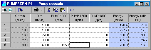
Fig. 4.21.16 Optimized pump scenario.

The total energy consumption is now reduced to 1673 MWh; that means a reduction of 4 %.

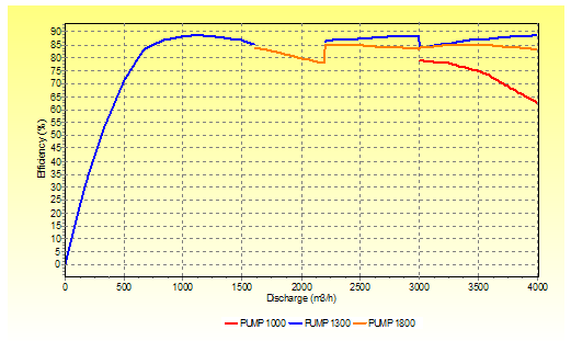
Fig. 4.21.17 Optimized pump scenario result.

Step 6: analyse a 24 hours period

Replace the Q_FREQ by the Q_PATTRN and specify the discharge pattern

Note: it is not necessary to connect the Q_PATTRN to the pumps

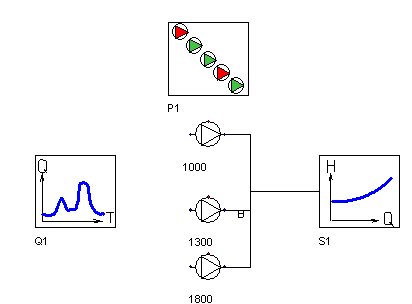
Fig. 4.21.18 Altered Wanda schematic.

Step 7: Specify data for Q_PATTRN

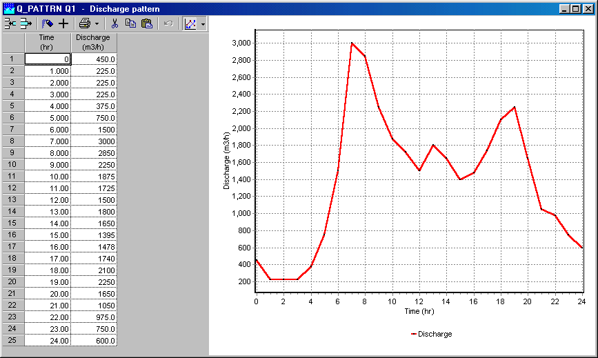
Fig. 4.21.19 Discharge pattern for the pumps.

Step 8: analyse the results

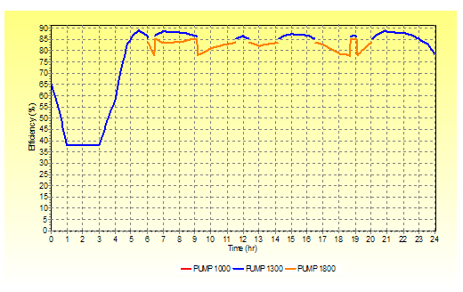
Fig. 4.21.20 Results of the changed discharge pattern for time versus efficiency.

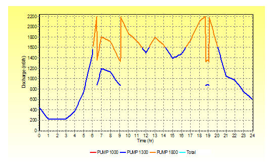
Fig. 4.21.21 Results of the changed discharge pattern for time versus discharge.

Advise: use for the low discharges (0 – 400 m³/h) a pump with lower capacity.