4.29. T-JUNCTION

Fig. 4.29.1 T-Junction

type label	description	active
T-straight	Three-node junction with the combined flow in the straight leg. Both straight legs have the same diameter	no
T-branch	Three-node junction with the combined flow in the branch. Both straight legs have the same diameter	no

Both components can be used for all kind of flow regimes in a 90 degree T‑junction. The difference between the two T-junctions has to do with the positive flow definition. The arrows in the symbol specify the positive direction of the flow (and the velocity).

The two different symbols allow the user to express his design (normal) flow scenario with positive flows. If he expects in the steady state the combined (total) flow in the straight part he may prefer the left symbol. A combined flow, coming into or out of the branch, gives preference to the right symbol.

4.29.1. Mathematical model

4.29.1.1. Positive flow definition

The definition for the positive direction of flow (and velocity) is important to understand the results in the property window. Each T-junction type has his own definition.

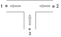
For the T-straight component the positive flow definition is defined in the left figure below.

Fig. 4.29.2 T-straight

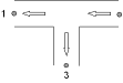
For the T-branch component (right figure) the positive flow definition for the first connection point is opposite to that of the T-straight component; for the two other connection points the positive flow definitions are the same as for the T-straight component.

Fig. 4.29.3 T-branch

4.29.1.2. Flow regimes

In the figures below all different flow regimes which can occur are listed and explained with a scheme with corresponding actual flow arrows. It is called straight flow if the total flow (in some literature also called: combined flow) is in one of the straight legs, branch flow means that the total flow is in the branch.

Fig. 4.29.4 Positive straight flow

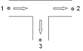
Fig. 4.29.5 Negative straight flow

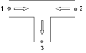
Fig. 4.29.6 Combining branch flow

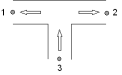
Fig. 4.29.7 Dividing branch flow

The sign of the discharge and velocity output (results) depends of the T-junction type chosen, but is independent of the flow regime definition. The example below will illustrate this.

The main flow is from West to East with a supply from the South. That means we are dealing with a combining straight flow with the combined flow in leg 2. The solution of the calculation for the T-straight model (positive Q) as well as the T-branch model (negative Q) is shown in the figures below.

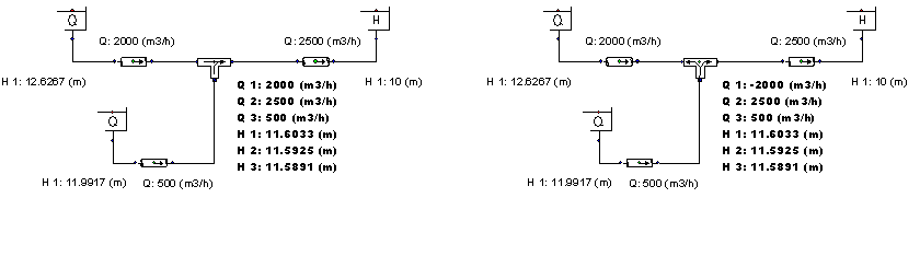
Fig. 4.29.8 Example solution with a T-straight model (positive Q) and a T-branch model (negative Q).

4.29.1.3. Equations

The head loss over a 3-node component depends on the distribution of the discharges and the area of the connected legs. The T-junction supports two different ways for retrieving the resistance coefficient Xi (ξ).

1. the head loss functions according to Idelchik’s Handbook [ref. 1]

2. user specified table with Xi depending on discharge ratio. These table values belong to a fixed area ratio.

Please note that the loss coefficients according to the handbooks apply to junctions with a certain minimum pipe length interval in between multiple junctions.

The head loss in 3-node components is a function of the combined flow in the combined leg, which is either one leg (1 or 2) of the straight part or the branch (leg 3). Including the continuity equation (no production or loss of mass in the component) the general set of the three equations of the T-junction is:

(4.29.1)\[f_{1}=Q_{1}-Q_{2}+Q_{3}=0\]

ΔH T-junction straight, combined flow in leg 2

(4.29.2)\[f_{2}=H_{1}-H_{2}-\xi_{12} \frac{Q_{2}\left|Q_{2}\right|}{2 g A_{2}^{2}}\]

ΔH T-junction straight, combined flow in leg 1

(4.29.3)\[f_{2}=H_{1}-H_{2}-\xi_{12} \frac{Q_{1}\left|Q_{1}\right|}{2 g A_{1}^{2}}\]

ΔH T-junction branch, combined flow in branch

(4.29.4)\[f_{2}=H_{3}-H_{1}-\xi_{31} \frac{Q_{3}\left|Q_{3}\right|}{2 g A_{3}^{2}}\]

Where:

Variable	Units
Q i = total discharge in leg i	[m3/s]
Hi = energy head in connect point i	[m]
Ai = pipe area leg i (leg with total flow)	[m2]
ξij = loss coefficient between point i and j	[-]

The subscripts (1), (2) and (3) correspond to the different legs. The subscript x at the discharge Q_x refers always to the leg in which the combined (total) flow Q occurs.

For positive straight dividing flow and negative straight combining flow, Q₁ will be taken into account. For positive straight combining flow and negative straight dividing flow, Q₂ will be taken into account.

4.29.1.4. Resistance coefficients based on formulas

The resistance coefficients based of formulas are taken from the Idelchik Handbook with the following restriction to the section areas:

(4.29.5)\[\begin{split}\begin{array}{l} A_{1}+A_{3}>A_{2} \\ A_{1}=A_{2} \end{array}\end{split}\]

For all different flow regimes the formulas used are described, and a table shows the ξ‑values for various area and discharge ratios. Note that all indices used in the formulas are based on positive flow.

Straight flow combining

For the straight leg, the resistance coefficient is calculated according to:

(4.29.6)\[\xi_{12} \approx 1.55 \frac{Q_{3}}{Q_{2}}-\left(\frac{Q_{3}}{Q_{2}}\right)^{2}\]

The table below shows the ξ12 values according to the formula above for various values of the discharge ratio.

Table 4.29.1 ξ₁₂ values for combining flow.

Q3/Q2	A3/A2
0.0	0.00
0.1	0.14
0.2	0.27
0.3	0.38
0.4	0.46
0.5	0.52
0.6	0.57
0.7	0.59
0.8	0.60
0.9	0.58
1.0	0.55

For the branch, the resistance coefficient ξ32 is calculated according to:

(4.29.7)\[\xi_{32}=A\left[1+\left(\frac{Q_{3}}{Q_{2}} \frac{A_{2}}{A_{3}}\right)^{2}-2\left(1-\frac{Q_{3}}{Q_{2}}\right)^{2}\right]\]

The coefficient A depends on the area and discharge ratios again. Table 3 shows the values.

Table 4.29.2 Values of the variable A.

A3/A2	≤ 0.35	> 0.35
Q3/Q2	0 – 1.0	≤ 0.4	> 0.4
A	1.0	\(0.9\left(1-\frac{Q_{3}}{Q_{2}}\right)\)	0.55

The table below shows the ξ32 values according to the formulas above for various values of the discharge and area ratios.

Table 4.29.3 ξ₃₂ values for combining flow.

		A3/A2
		0.1	0.2	0.3	0.4	0.5	0.6	0.7	0.8	0.9	1.0
Q3/Q2	0.0	‑1.00	‑1.00	‑1.00	‑0.90	‑0.90	‑0.90	‑0.90	‑0.90	‑0.90	‑0.90
	0.1	0.38	‑0.37	‑0.51	‑0.45	‑0.47	‑0.48	‑0.49	‑0.49	‑0.49	‑0.49
	0.2	3.72	0.72	0.16	‑0.02	‑0.09	‑0.12	‑0.14	‑0.16	‑0.17	‑0.17
	0.3	9.02	2.27	1.02	0.37	0.24	0.17	0.13	0.10	0.08	0.07
	0.4	16.28	4.28	2.06	0.69	0.50	0.39	0.33	0.29	0.26	0.24
	0.5	25.50	6.75	3.28	1.13	0.83	0.66	0.56	0.49	0.44	0.41
	0.6	36.68	9.68	4.68	1.61	1.17	0.92	0.78	0.68	0.62	0.57
	0.7	49.82	13.07	6.26	2.14	1.53	1.20	1.00	0.87	0.78	0.72
	0.8	64.92	16.92	8.03	2.71	1.91	1.48	1.22	1.06	0.94	0.86
	0.9	81.98	21.23	9.98	3.32	2.32	1.78	1.45	1.24	1.09	0.98
	1.0	101.00	26.00	12.11	3.99	2.75	2.08	1.67	1.41	1.23	1.10

Straight flow dividing

For the straight leg the resistance coefficient is given using the following formula:

(4.29.8)\[\xi_{12}=\tau_{12} \frac{Q_{3}}{Q_{1}}\]

where τ₁₂ depends on the area and discharge ratios as given in Table 4.29.4.

Table 4.29.4 Values of \(\tau_{12}\)

A3/A1	≤ 0.4	0.4
Q3/Q1	0-1.0	≤ 0.5	>0.5
τ12	0.4 (Q3/Q1)	0.2(2Q3/Q1 – 1)	0.3(2Q3/Q1 – 1)

Table 4.29.5 shows the ξ12 values according to the formula above for various values of discharge ratios.

Table 4.29.5 Values of \(\xi_{12}\) for dividing flow

		A3/A1
		0.1	0.2	0.3	0.4	0.5	0.6	0.7	0.8	0.9	1.0
Q3/Q1	0.0	0.00	0.00	0.00	0.00	0.00	0.00	0.00	0.00	0.00	0.00
	0.1	0.00	0.00	0.00	0.00	-0.02	-0.02	-0.02	-0.02	-0.02	-0.02
	0.2	0.02	0.02	0.02	0.02	-0.02	-0.02	-0.02	-0.02	-0.02	-0.02
	0.3	0.04	0.04	0.04	0.04	-0.02	-0.02	-0.02	-0.02	-0.02	-0.02
	0.4	0.06	0.06	0.06	0.06	-0.02	-0.02	-0.02	-0.02	-0.02	-0.02
	0.5	0.10	0.10	0.10	0.10	0.00	0.00	0.00	0.00	0.00	0.00
	0.6	0.14	0.14	0.14	0.14	0.04	0.04	0.04	0.04	0.04	0.04
	0.7	0.20	0.20	0.20	0.20	0.08	0.08	0.08	0.08	0.08	0.08
	0.8	0.26	0.26	0.26	0.26	0.14	0.14	0.14	0.14	0.14	0.14
	0.9	0.32	0.32	0.32	0.32	0.22	0.22	0.22	0.22	0.22	0.22
	1.0	0.40	0.40	0.40	0.40	0.30	0.30	0.30	0.30	0.30	0.30

The resistance coefficient ξ13for the branch is calculated using the following formula:

For A₃/A₁ ≤ 2/3:

(4.29.9)\[\xi_{13}=A^{\prime}\left[1+\left(\frac{Q_{3}}{Q_{1}} \frac{A_{1}}{A_{3}}\right)^{2}\right]\]

For A₃/A₁ = 1 (up to velocity ratio to v3/v1≈2.0):

(4.29.10)\[\xi_{13}=A^{\prime}\left[1+0.3\left(\frac{Q_{3}}{Q_{1}} \frac{A_{1}}{A_{3}}\right)^{2}\right]\]

The values of A’ are given in Table 4.29.6.

Table 4.29.6 Values for \(A'\) dividing flow.

A3/A1	≤ 0.35	> 0.35
Q3/Q1	≤ 0.4	> 0.4	≤ 0.6	> 0.6
A’	1.1 – 0.7 Q3/Q1	0.85	1.0 – 0.65 Q3/Q1	0.6

Table 4.29.7 shows the ξ13 values according to the formulas above for various values of discharge and area ratio.

Table 4.29.7 Values for \(\xi_{13}\)

		A3/A1
		0.1	0.2	0.3	0.4	0.5	0.6	0.7	0.8	0.9	1
Q3/Q1	0	1.10	1.10	1.10	1.00	1.00	1.00	1.00	1.00	1.00	1.00
	0.1	1.34	1.11	1.06	0.95	0.95	0.94	0.94	0.94	0.94	0.94
	0.2	2.11	1.25	1.09	0.94	0.91	0.90	0.89	0.89	0.88	0.88
	0.3	3.29	1.49	1.16	0.94	0.89	0.87	0.85	0.84	0.83	0.83
	0.4	4.76	1.80	1.26	0.96	0.88	0.84	0.81	0.80	0.78	0.78
	0.5	7.23	2.44	1.56	0.99	0.88	0.82	0.78	0.75	0.74	0.73
	0.6	10.03	3.15	1.87	1.02	0.87	0.79	0.74	0.71	0.69	0.68
	0.7	13.35	3.97	2.24	1.15	0.95	0.85	0.78	0.74	0.71	0.69
	0.8	17.17	4.93	2.66	1.32	1.06	0.92	0.84	0.78	0.74	0.72
	0.9	21.51	6.01	3.14	1.51	1.18	1.00	0.90	0.83	0.78	0.75
	1	26.35	7.23	3.68	1.73	1.32	1.10	0.97	0.88	0.82	0.78

Branch flow combining

WANDA calculates the head loss coefficients for each leg (ξ31 and ξ32 ) from the following formula:

(4.29.11)\[\xi_{31}=A\left\{1+\left(\frac{A_{3}}{A_{1}}\right)^{2}+3\left(\frac{A_{3}}{A_{1}}\right)^{2}\left[\left(\frac{Q_{1}}{Q_{3}}\right)^{2}-\left(\frac{Q_{1}}{Q_{3}}\right)\right]\right\}\]

In which A is the same factor as used in the T-junction straight combining (table 3).

Table 4.29.8 shows the ξ31 values according to the formulas above for various values of discharge and area ratio (identical for ξ32 in leg 2).

Table 4.29.8 Values for \(\xi_{13}\) and \(\xi_{32}\).

		A1/A3
		0.1	0.2	0.3	0.4	0.5	0.6	0.7	0.8	0.9	1.0
Q1/Q3	0.0	101.00	26.00	12.11	6.52	4.50	3.40	2.74	2.31	2.01	1.80
	0.1	74.00	19.25	9.11	4.51	3.18	2.45	2.02	1.73	1.54	1.40
	0.2	53.00	14.00	6.78	3.06	2.22	1.76	1.48	1.30	1.18	1.09
	0.3	38.00	10.25	5.11	2.09	1.56	1.28	1.11	0.99	0.92	0.86
	0.4	29.00	8.00	4.11	1.48	1.14	0.96	0.85	0.78	0.73	0.69
	0.5	26.00	7.25	3.78	1.41	1.10	0.93	0.83	0.76	0.72	0.69
	0.6	29.00	8.00	4.11	1.51	1.17	0.98	0.86	0.79	0.74	0.70
	0.7	38.00	10.25	5.11	1.82	1.36	1.12	0.97	0.87	0.80	0.75
	0.8	53.00	14.00	6.78	2.34	1.69	1.34	1.13	1.00	0.90	0.84
	0.9	74.00	19.25	9.11	3.06	2.16	1.67	1.37	1.18	1.05	0.95
	1.0	101.00	26.00	12.11	3.99	2.75	2.08	1.67	1.41	1.23	1.10

Branch flow dividing

WANDA calculates the head loss coefficients for each leg (ξ31 and ξ32 ) from the following formula:

(4.29.12)\[\xi_{31}=1+k\left(\frac{Q_{1}}{Q_{3}} \frac{A_{3}}{A_{1}}\right)^{2}\]

In which k is 0.3 valid for welded tees.

Table 4.29.9 shows the ξ31 values according to the formulas above for various values of discharge and area ratio (identical for ξ32 in leg 2).

Table 4.29.9 ξ₃₁ and ξ₃₂ values for dividing branch flow

		A1/A3
		0.1	0.2	0.3	0.4	0.5	0.6	0.7	0.8	0.9	1.0
Q1/Q3	0.0	1.00	1.00	1.00	1.00	1.00	1.00	1.00	1.00	1.00	1.00
	0.1	1.30	1.08	1.03	1.02	1.01	1.01	1.01	1.00	1.00	1.00
	0.2	2.20	1.30	1.13	1.08	1.05	1.03	1.02	1.02	1.01	1.01
	0.3	3.70	1.68	1.30	1.17	1.11	1.08	1.06	1.04	1.03	1.03
	0.4	5.80	2.20	1.53	1.30	1.19	1.13	1.10	1.08	1.06	1.05
	0.5	8.50	2.88	1.83	1.47	1.30	1.21	1.15	1.12	1.09	1.08
	0.6	11.80	3.70	2.20	1.68	1.43	1.30	1.22	1.17	1.13	1.11
	0.7	15.70	4.68	2.63	1.92	1.59	1.41	1.30	1.23	1.18	1.15
	0.8	20.20	5.80	3.13	2.20	1.77	1.53	1.39	1.30	1.24	1.19
	0.9	25.30	7.08	3.70	2.52	1.97	1.67	1.50	1.38	1.30	1.24
	1.0	31.00	8.50	4.33	2.88	2.20	1.83	1.61	1.47	1.37	1.30

4.29.2. T-Junction properties

The input properties of both T-junction are not exactly the same. The differences are located in the sequence of the Xi tables and the description labels for input tables and output properties. The input and output properties for both types are specified below.

4.29.2.1. Properties T-junction straight

Input properties T-junction straight

Description	input	unit	range	default	Remarks
Diameter straight leg	Real	[mm]
Diameter branch leg	Real	[mm]
Xi method	Formula Tables			Formula
Xi tables valid for	Combining Dividing All				Only when Xi method = Tables
Xi straight flow combining, leg straight	Table (ξ12)				if Xi tables = Combining or All
Xi straight flow combining, leg branch	Table (ξ32)				if Xi tables = Combining or All
Xi straight flow dividing, leg straight	Table (ξ12)				if Xi tables = Dividing or All
Xi straight flow dividing, leg branch	Table (ξ13)				if Xi tables = Dividing or All
Xi branch flow combining, leg 1	Table (ξ13)				if Xi tables = All
Xi branch flow combining, leg 2	Table (ξ23)				if Xi tables = All
Xi branch flow dividing, leg 1	Table (ξ31)				if Xi tables = All
Xi branch flow dividing, leg 2	Table (ξ32)				if Xi tables = All

With the tables for the Xi-values it is possible to choose user-defined loss coefficients, for instance for a certain kind of T-junction with rounded angles. The user has to specify a set of loss coefficient values related to the discharge ratio between the side and combined branch. If the user does not specify both combining and dividing Xi-tables, WANDA uses the formulas according to the Idelchik handbook for the unspecified flow regimes.

Example of Xi table; straight flow combining, leg branch (ξ32)

valid for Area ratio = 0.5

Discharge ratio [-]	Xi [-]
0.0	0.90
0.2	0.12
0.4	0.39
0.6	0.92
0.8	1.48
1.0	2.08

Component specific output T-junction straight

Loss coefficient straight [-]	The ξ12 for positive flow and ξ21 for negative flow In case of branch flow regime this is the ξ31 coefficient
Loss coefficient branch [-]	The ξ13 for positive flow and ξ31 for negative flow In case of branch flow regime this is the ξ32 coefficient
Head loss straight [m]	The ΔH12 for positive flow and ΔH21 for negative flow In case of branch flow regime this is the ΔH13 for combining and ΔH31 for dividing flow
Head loss branch [m]	The ΔH13 for positive flow and ΔH31 for negative flow In case of branch flow regime this is the ΔH23 for combining and ΔH32 for dividing flow

Component messages T-junction straight

Message	Type	Explanation
Combining	Info	Positive straight flow	Negative straight flow
Dividing	Info	Positive straight flow	Negative straight flow
Branch combining	Info
Branch dividing	info

With the tables for the Xi-values it is possible to choose user-defined loss coefficients, for instance for a certain kind of T-junction with rounded angles. The user has to specify a set of loss coefficients values related to the discharge ratio between the side and combined branch. If the user does not specify both combining and dividing Xi-tables, WANDA uses the formulas according to the Idelchik handbook for the unspecified flow regimes.

NOTE: The numbering of the branches in the literature is not always consistent with the WANDA definition as given under ‘Mathematical Model’ above. The Miller Handbook for instance indicates the side branch with 1, the straight branch with 2 and the combined one as 3.

Furthermore please note that there is a discontinuity when the flow in one of the legs goes through zero. This might lead to unstable behaviour.

4.29.2.2. Properties T-junction branch

Input properties T-junction branch

Description	input	unit	range	default	Remarks
Diameter straight leg	Real	[mm]
Diameter branch leg	Real	[mm]
Xi method	Formula Tables			Formula
Xi tables valid for	Combining Dividing All				Only when Xi method = Tables
Xi branch flow combining, leg 1	Table (ξ13)				if Xi tables = Combining or All
Xi branch flow combining, leg 2	Table (ξ23)				if Xi tables = Combining or All
Xi branch flow dividing, leg 1	Table (ξ31)				if Xi tables = Dividing or All
Xi branch flow dividing, leg 2	Table (ξ32)				if Xi tables = Dividing or All
Xi straight flow combining, leg straight	Table (ξ12)				if Xi tables = All
Xi straight flow combining, leg branch	Table (ξ32)				if Xi tables = All
Xi straight flow dividing, leg straight	Table (ξ12)				if Xi tables = All
Xi straight flow dividing, leg branch	Table (ξ13)				if Xi tables = All

Component specific output T-junction branch

Loss coefficient 1 [-]	The ξ31 for dividing flow and ξ13 for combining flow In case of straight flow regime this is the ξ12 or ξ21 coefficient
Loss coefficient 2 [-]	The ξ32 for dividing flow and ξ23 for combining flow In case of straight flow regime this is the ξ32 or ξ23 coefficient
Head loss 1 [m]	The ΔH31 for dividing flow and ΔH13 for combining flow In case of straight flow regime this is the ΔH12 or ΔH21
Head loss 2 [m]	The ΔH32 for dividing flow and ΔH23 for combining flow In case of straight flow regime this is the ΔH32 or ΔH23

Component messages T-junction branch

Message	Type	Explanation
Branch combining	Info
Branch dividing	info
Combining straight	Info	Positive straight flow	Negative straight flow
Dividing straight	Info	Positive straight flow	Negative straight flow

With the tables for the Xi-values it is possible to choose user-defined loss coefficients, for instance for a certain kind of T-junction with rounded angles. The user has to specify a set of loss coefficients values related to the discharge ratio between the side and combined branch. If the user does not specify both combining and dividing Xi-tables, WANDA uses the formulas according to the Idelchik handbook for the unspecified flow regimes.

NOTE: The numbering of the branches in the literature is not always consistent with the WANDA definition as given under ‘Mathematical Model’ above. The Miller Handbook for instance indicates the side branch with 1, the straight branch with 2 and the combined one as 3.

Furthermore please note that there is a discontinuity when the flow in one of the legs goes through zero. This might lead to unstable behaviour.