6.12. Pipe

Fig. 6.12.1 Schematic picture of the Heat Pipe component.

Fall type

Type label	Description	Active
Heat pipe	Pressurised pipe	Yes

6.12.1. Mathematical model

6.12.1.1. Fluid equations

The pipe is the primary component in WANDA to simulate the pressure wave propagation during transient simulations. In WANDA Heat, the pipe is also used to simulate the advection and radial transfer of heat in the system.

The PIPE is considered as a fall type. In steady-state the pressure loss is modelled by the following equations:

(6.12.1)\[\frac{p_1}{\rho_1g} - \frac{p_2}{\rho_2g} + z_1 - z_2 = \frac{8\lambda}{LD^5g\rho^2\pi^2}|\dot{m}|\dot{m}\]

(6.12.2)\[\dot{m}_1 - \dot{m}_2 = 0\]

with:

variable	Description	Units
\(p_{1}, p_{2}\)	Pressure at node 1 and node 2	Pa
\(z_{1}, z_{2}\)	Height at node 1 and node 2	m
\(f\)	Friction factor	-
\(D\)	Inner diameter of the pipe	m
\(\bar{\rho}=\frac{\rho_{1}+\rho_{2}}{2}\)	Average density	kg/m3
\(g\)	Gravitational acceleration	m/s2
\(L\)	Length of the pipe	m
\(\dot{m}\)	Mass flow rate through the pipe	kg/s

WANDA calculates the friction factor, f, iteratively using the Darcy-Weisbach wall roughness, k, which is explained in Theoretical friction models (Darcy-Weisbach). In Transient Mode, the friction factor is recalculated each time step using a quasi-steady approach.

The wave propagation speed is calculated based on pipe and fluid properties (analogous to the Liquid pipe with “calculation mode” set to “waterhammer”). Details about the wave propagation and the equations involved are discussed in Theory on waterhammer pipes in Theoretical and mathematical background.

Note: only a circular cross section is supported in WANDA Heat.

6.12.1.2. Heat equations

The heat transfer in the pipe is calculated by dividing the pipe in elements, see Fig. 6.12.2.

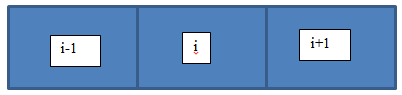
Fig. 6.12.2 Subdivision of pipe in elements for the temperature calculations

The temperature is calculated for each element, \(i\). In the case of positive flow, the following energy balance holds:

(6.12.3)\[\frac{ \rho_i c_{p,i} V \left( T_i^{t + \Delta t} - T_i^{t} \right) }{\Delta t} = \left( c_p \dot{m} T \right)_{i-1}^{t} - \left( c_p \dot{m} T \right)_{i}^{t} - Q_{loss} + fr \left( \frac{\xi}{L} + \frac{f}{D} \right) \frac{\dot{m}_i^2 \lvert \dot{m}_i \rvert}{2\rho_i^2 A_i^2} ds\]

with:

variable	Description	Units
\(\rho\)	Fluid density	kg/m3
\(c_p\)	Specific heat	J/kg/K
\(V\)	Volume of the observed element	m3
\(T\)	Temperature	K
\(\dot{m}\)	Mass flow rate	kg/s
\(Q_{loss}\)	Heat loss	W
\(\xi\)	Local loss coefficient	-
\(L\)	Length of the entire pipe	m
\(f\)	Friction coefficient	-
\(A\)	Area of the pipe	m2
\(fr\)	Fraction of friction converted to heat loss	-
\(ds\)	Element length	m

Note that the division must be determined before a steady-state simulation can be run. The division of the pipes in elements depends on the chosen calculation mode for the pipes. The water hammer grid is used for water hammer pipes, which is explained in Section 3.3.2.1.

In a rigid column pipe or in engineering mode, the length of an element of the grid is calculated from:

(6.12.4)\[ds = \frac{L}{n}\]

variable	Description	Units
\(n\)	Number of internal grid cells	-

The number of grid cells is an input for the user. The Courant number should be smaller than 1 for numerical stability. This is:

(6.12.5)\[CFL = \frac{v dt}{ds} < 1\]

A warning is given when this criterium is not met. The user can then adapted either the number of elements of the pipe or reduce the time step.

Moreover, a super bee flux limiter scheme is implemented to ensure conservation of steep temperature fronts [5].

The heat loss defined by equation (6.12.3) includes all the heat losses to the surrounding. The heat is transported from the fluid through the one or multiple pipe wall layers to the surrounding subsoil. The heat loss of an element of the pipe is defined by [6] [7]:

(6.12.6)\[Q_{loss} = ds\left( U_{1 i} - U_{2 i} \right)\left( T_{i} - T_{s} \right) + ds U_{2 i}\left( T_{i} - T_{ri} \right)\]

with:

variable	Description	Units
\(U_{1 i}\)	Combined heat loss coefficient of the ith element of the pipe	W/m/K
\(U_{2 i}\)	Heat loss coefficient of the ith element of the pipe due to an adjacent pipe	W/m/K
\(T_s\)	Temperature of the surrounding subsoil	K
\(T_r\)	Temperature of the ith element of the adjacent pipe	K

The heat loss coefficients are, respectively, defined by:

(6.12.7)\[U_i = \frac{R_{f} + R_{s} + R_{l}}{\left(R_{f} + R_{s} + R_{l} \right)^2 - R_m^2}\]

(6.12.8)\[U_r = \frac{R_{m}}{\left(R_{f} + R_{s} + R_{l} \right)^2 - R_m^2}\]

in which

variable	Description	Units
\(R_f\)	Thermal resistance of the fluid	K/W/m
\(R_l\)	Thermal resistance of all pipe wall layers	K/W/m
\(R_s\)	Thermal resistance of the subsoil	K/W/m
\(R_m\)	Thermal resistance due to influence adjacent pipes	K/W/m

How the different resistance factor can be calculated is discussed in the following sections.

Resistance of heat transfer through the fluid

The heat transport in the fluid is determined by the flow regime (laminar or turbulent).

For laminar flow the following conditions apply [8] [9]:

(6.12.9)\[\begin{split}Nu = \begin{cases} 3.66, & \text{if } Gz > 0.1 \\ 1.62 Gz^{-\frac{1}{3}}, & \text{if } Gz < 0.05 \end{cases}\end{split}\]

with:

variable	Description	Units
\(Nu\)	The dimensionless Nusselt number	-
\(Gz\)	The dimensionless Greatz number	-

The Greatz-number is defined as:

(6.12.10)\[Gz = \frac{a}{Dv}\]

with:

variable	Description	Units
\(a\)	Thermal diffusion coefficient	m2/s
\(D\)	Inner diameter of the pipe	m
\(v\)	Fluid velocity	m/s

The thermal resistance, \(R_f\), can be calculated as follows:

(6.12.11)\[R_f = \frac{1}{Nu \lambda \pi}\]

with:

variable	Description	Units
\(\lambda\)	Heat conductivity coefficient	W/m/K

The Nusselt number for turbulent flow (\(Re > 10^4\) and \(Pr \geq 0.7\)) is defined by [10]:

(6.12.12)\[Nu = 0.027Re^{0.8}Pr^{0.33}\]

with:

variable	Description	Units
\(Pr\)	Dimensionless Prandtl number	-

The Prandtl-number is defined as:

(6.12.13)\[Pr = \frac{\nu}{a}\]

with:

variable	Description	Units
\(\nu\)	Kinematic viscosity of the fluid	m2/s

Thus the equations given above can be used to calculate the resistance of the fluid for heat transfer.

Heat transfer through the pipe wall layers

For a general radial system, the heat transfer coefficient through a layer of material, \(j\), can be calculated from:

(6.12.14)\[R_j = \frac{ \ln\frac{D_{j,out}}{D_{j,in}}}{2 \lambda_j}\]

with:

variable	Description	Units
\(\lambda_j\)	Heat conductivity coefficient of the layer \(j\)	W/m/K
\(D_{j,in}\)	Inner diameter of the layer \(j\)	m
\(D_{j,out}\)	Outer diameter of the layer \(j\)	m

Fig. 6.12.3 shows the definitions of the parameters of (6.12.14).

Fig. 6.12.3 Definition of the heat transfer coefficient in a radial system.

The thermal resistance of all pipe wall layers, \(R_{l}\), can be calculated with:

(6.12.15)\[ R_{l} = \sum R_j\]

Heat transfer through the subsoil

The heat resistance of the subsoil, \(R_s\), when there is no adjacent pipe, is given by [6]:

(6.12.16)\[R_s = \frac{1}{2 \pi \lambda_s} \ln \left[ \frac{2H}{D_c} + \sqrt{\left( \frac{2H}{D_c} \right)^2 -1} \right]\]

with:

variable	Description Units
\(R_s\)	Heat resistance of the subsoil	m K/W
\(\lambda_s\)	Thermal conductivity of the subsoil	W/m/K
\(H\)	Corrected depth of the pipe centre (see eq. (6.12.17))	m
\(D_c\)	Outer diameter of the pipe	m

The corrected depth of the pipe can be calculated as:

(6.12.17)\[H = H^\prime + \frac{\lambda_s}{h_{s}} + \frac{D_c}{2}\]

with:

variable	Description	Units
\(H^{\prime}\)	Thickness of the subsoil layer on top of the pipe	m
\(h_{s}\)	Heat transfer coefficient at the soil surface	W/m2/K

Influence of adjacent pipe

If there is a adjacent pipe, the heat resistance of the subsoil, can be calculated from:

(6.12.18)\[R_{s} = \frac{1}{2\pi\lambda_{s}}\left\lbrack \ln\left( \frac{4H}{D_{c}} \right) \right\rbrack\]

Additionally, the influence of adjacent pipes can be considered (see Fig. 6.12.4). Adjacent pipes will influence the temperature in the ground and should, therefore, be considered simultaneously. Note that adjacent pipes must have the same length and number of elements in WANDA. The heat resistance due to the influence of a nearby pipe, \(R_{m}\), is given by:

(6.12.19)\[R_m = \frac{1}{2\pi\lambda_s} \left\lbrack \ln\left( \sqrt{ 1 + \left(\frac{2H}{D_{c}} \right)^2}\right) \right\rbrack\]

with:

variable	Description	Units
\(d\)	Distance between two adjacent pipe centres	m

Fig. 6.12.4 Heat loss from two adjacent pipe.

6.12.1.3. Heat by tracing

Heat tracing can be used to maintain process temperatures for piping. Equation (6.12.3) is then modified to:

(6.12.20)\[\frac{ \rho_i c_{p,i} V \left( T_i^{t + \Delta t} - T_i^{t} \right) }{\Delta t} = \left( c_p \dot{m} T \right)_{i-1}^{t} - \left( c_p \dot{m} T \right)_{i}^{t} - Q_{loss} + fr \left( \frac{\xi}{L} + \frac{f}{D} \right) \frac{\dot{m}_i^2 \lvert \dot{m}_i \rvert}{2\rho_i^2 A_i^2} ds + Q_{tracing} ds\]

with:

variable	Description	Units
\(Q_{tracing}\)	Heat provided by tracing per unit length	W/m

6.12.1.4. Thermal expansion

Expansion of the pipe

Thermal expansion of the pipe is not taken into account. The assumption of negligble thermal expansion does not hold for a system that heats up or cools down significantly. This significant change of temperature can be realized over a short or long duration of time. Consequently, a Wanda model with a pipe that experiences a significant temperature change over the duration of the simulation should be interpreted with care.

The expansion of a pipe (\(\Delta L\)) can be estimated with:

(6.12.21)\[\Delta L = \alpha L \Delta T\]

with the thermal expansion coefficient of the pipe material (\(\alpha\)), the length of the pipe (\(L\)), and the temperature variation (\(\Delta T\)). The expansion of a pipe is negligble in a typical Wanda simulation. The uncertainty due to thermal expasion of the pipe can be estimated by considering the total variation in temperature per pipe over the duration of the Wanda simulation.

For example, a steel pipe with a thermal expansion coefficient of \(\alpha = 12.5 \times 10^{-6}\) °C would require a temperature increase over the duration of the simulation of \(\Delta T = 800\) °C to experience a relative length change of \(\Delta L / L \approx 1 \%\).

Expansion of the fluid

Thermal expansion of the fluid is neglected, as the volumetric thermal expansion of a fluid is negligible for relatively small changes of the temperature. The density of a fluid, at constant pressure and small changes of temperature, is given by:

(6.12.22)\[\rho = \frac{\rho_{T_0}}{1 + \alpha \Delta T}\]

with the density (\(\rho_{T_0}\)), and thermal expansion (\(\alpha\)) of the fluid at a reference temperature close to the required temperature.

Mass (\(m = \rho V\)) is not conserved when the temperature increases, as the fluid volume does not change (i.e., \(V_1 = V_2\) ) due to the neglected thermal expansion. On the other hand, the fluid density does change (i.e., \(\rho_2 = \rho_1 + \Delta \rho\)) which should result in a change of mass (i.e., \(\rho_1 /(\rho_1 + \Delta \rho) = m_1/(m_1 + \Delta m)\)). However, the error introduced by neglecting the thermal expansion is negligble for systems that do not heat up or cool down significantly over the duration of the Wanda simulation. The relative density change over the extend of a Wanda simulation can be used as a measure for the uncertainty due to thermal expansion.

For example, the relative density change of water (i.e., \(\alpha = 4.57 \times 10^{-4}\) 1/°C at 50 °C) with a temperature increase of \(\Delta T = 60\) °C will be \((\rho + \Delta \rho)/\rho = 1 / (1 + \alpha \Delta T) \approx 0.97\).

6.12.1.5. Additional losses

If several local losses (like bends, Tee’s etc) exist in a pipe section, you can combine them in the pipe model (neglecting the exact position). Combining them can be done in 3 different ways, using either:

• the ξ-annotation (e.g. for one elbow ξ_elbow is about 0.2, hence for 5 elbows the combined ξ-value is 1.0)

• the equivalent length annotation (for an elbow L_eq is about 15 \(D\))

• a percentage relative to the calculated loss in the pipe itself.

6.12.1.6. Geometry

For more information about the geometry, we refer to the explanation in the Liquid module: Section 4.18.2.3.

6.12.2. Heat pipe

6.12.2.1. Hydraulic specifications

Input properties

Description	Input	SI-units	Remarks
Inner diameter	real	[m]
Wall roughness	real	[mm]
Calculation mode	Waterhammer Rigid column		Only in transient mode, default = Rigid column
Wave speed mode	Physical Specified		Only if Calculation mode = Waterhammer, default = Physical
Wall thickness	real	[m]	Only in transient mode and with Wave speed mode = Physical
Young’s modulus	real	[N/m2]	Only in transient mode and with Wave speed mode = Physical
Specified wave speed	real	[m/s]	Only in transient mode and with Wave speed mode = Specified
Number of pipe elements	integer	[-]	Only in engineering mode or with calculation mode Rigid column
Geometry input	Length l-h xyz xyz diff	[-]	Default = Length
Length	real	[m]	if Geometry input = Length
Profile	table		if Geometry input = L-h, xyz or xyz diff
Upper limit pressure	real	[N/m²]	Only for post processing, not needed for calculation
Lower limit pressure	real	[N/m²]	Only for post processing, not needed for calculation
Additional losses	None Xi Length Percentage	[-]	Default = None
Local losses coeff	real	[-]	If Additional losses = Xi
Additional length	real	[m]	If Additional losses = Length
Add. loss percentage	real	[%]	If Additional losses = Percentage
Fraction gen. heat to fluid	real	[%]
Heat transf. in fluid	yes no	[-]
Heat transf. input	Value Table diameter Table thickness	[-]
Heat transf coef	real	[W/m²/K]	if Heat transf input = Value
Heat transf. table diameter	table		if Heat transf input = table diameter, see remark below the table
Heat transf. table thickness	table		if Heat transf input = table thickness, see remark below the table
Heat trans. ground	Yes No	[-]	if Heat transf input = table diameter or table thickness
Ground coverage	real	[m]	If Heat trans. Ground = yes
Thermal conductivity of ground	real	[W/m/K]	If Heat trans. Ground = yes
Heat transfer coefficient at ground surface	real	[W/m2/K]	If Heat trans. Ground = yes
Adjacent pipe	Yes No		If Heat trans. Ground = yes
Pipe pair number	integer	[-]	If Adjacent pipe = yes see remark below the table
Distance between centre of the pipes	real	[m]	if adjacent pipe = yes
Heat by tracing	Constant value Time table		Default = Constant value
Value heat by tracing	real	[W/m]	if Heat by tracing = Constant value
Table heat by tracing	table	[-]	if Heat by tracing = Tine table
Ambient temperature	real	[°C]	Controllable with control component
Use action table	No Yes	[-]
Action table	Time vs Temperature	[-]	If Use action table = yes
Location	real	[m]	If empty, chart button creates a location series If filled in, chart button creates a time series for nearest internal calculation node

Remarks

The location charts of “Pressure” and “Head” shows the specified limits only if they are filled in. It is possible to specify these values after the simulation. If these fields are not visible, first check the “Upper/Lower limits in pipes” fields in the Mode & option window. You may change these values without re-calculating the case. In the heat domain, the change in the maximum head criterion due to changing density is not taken into account.

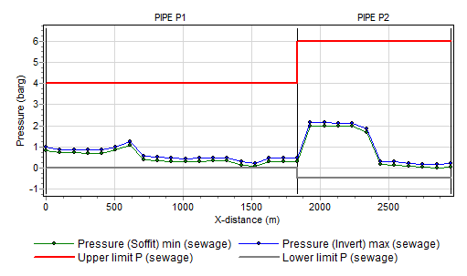
Fig. 6.12.5 Pressure location chart with additional pressure rating series

Note that the reference for the pressure output (centre line / soffit (top) / invert (bottom) is defined in the Mode & options window.

The main output properties like “Discharge” and “Pressure” contains output values in each calculation node or element in the pipe. That means that the chart button automatically creates a location chart. If you want a time chart in a particular pipe node you have to specify the location in the “Location” field.

To have direct access to the first and last node of the pipe (corresponding with the left and right H-node) you may extend the output property list with these points by checking the field “Connect point output in pipes” in “Modes & Options” (ctrl-m). Pressing the chart button in these additional fields automatically generates a time series chart.

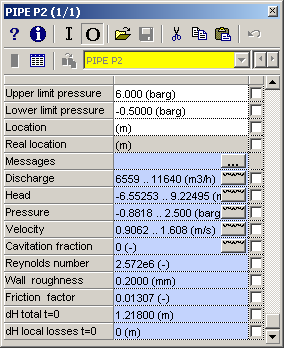
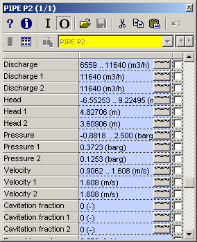
Two appearances of output properties window depending on Mode & Options setting “Connect point output in pipes”.

Heat transfer coefficient

The user has different options to fill in the heat transfer coefficient:

• Value, the user can now specify one value for the complete heat transfer from the fluid to the surroundings.

• Table diameter, the table should be filled with the outer diameter and heat conductivity coefficient of each layer of the pipeline. starting with the most inner layer.

• Table thickness, the table should be filled with the thickness and heat conductivity coefficient of each layer of the pipeline. Starting with the most inner layer.

For the second and the third option the user should fill the table for all the materials of which the pipe consists.

Adjacent pipe property.

The user needs to specify pairs of pipes in the model via the pipe number input property to include the effect of an adjacent pipe. This value should be an unique number for each pair of pipes. If the same number is given for more than two pipes an error message is given.

The user should ensure that the number of elements in both pipes is the same. If this is not the case an error message is generated.

6.12.2.2. Component specific output

Output	Description
Wave speed [m/s]	Wave propagation speed based on fluid properties and pipe properties
Pipe element count [-]	Amount of elements of same length in which pipe is divided.
Adapted wave speed [m/s]	Wave speed is adapted in such way that a integer number of elements (minimal 1) fit in the total length
Deviation adapted [%]	Ratio between wave speed and adapted wave speed. Must be less than 25% for a valid computation
H-node height check	Input validation between H-node height with corresponding pipe node elevation. OK means the difference is less than 0,5 D, otherwise “Warning” is displayed.
Real location [m]	If a location is specified the nearest (internal) calculation node will be selected. The real location is the location of this calculation node.
Cavitation fraction [-]	Ratio between cavitation volume and element volume Must be less than 20% for valid range of cavitation algorithm
Friction heat [W]	The generated heat due to friction with the pipe wall
Heat loss [W]	Heat radiated to the surroundings through the pipe wall
Total heat gain [W]	Total heat gain including effect of ‘fraction generated heat to fluid’ parameter (heat actually absorbed by the fluid)
Ambient temperature [°C]	The friction factor is used in the calculation of the head loss. This factor is calculated iteratively based on the wall roughness.
Friction factor [-]	The friction factor is used in the calculation of the head loss. This factor is calculated iteratively based on the wall roughness.
Kinematic viscosity [m2/s]	The kinematic viscosity.

6.12.2.3. Actions

The action table (control connection) of this component controls the ambient temperature as function of time.